qcrc_main <- import(here("data", "QCRC_FINAL_Deidentified.xlsx")) %>%
             mutate(BMI = as.numeric(BMI),
                    ICU_LOS = as.numeric(ICU_LOS))
neo <- import("https://www.kaggle.com/api/v1/datasets/download/zahrazolghadr/neonatal-hypothermia")
options(scipen = 999) #This sets the numer of digits for p-values so that we can avoid scientific notationInferential Statistics and Modeling Review
Learning objectives:
Develop a statistical hypothesis for a given research question
Identify appropriate statistical test for a given hypothesis
Implement meaningful code to model data and answer research questions
Data
Helpful Package
The janitor package can be helpful in expediting the initial data cleaning that comes along with analysis. One particular function I want to draw your attention to is clean_names as it will:
replace spaces with underscores
make all letters lowercase
remove non-standard characters
Janitor Example
Currently the names are a bit of a mess:
[1] "Patient_DEID"     "Decatur_Transfer" "Age"              "Female"
[5] "Race"             "Died"             "30D_Mortality"
Let’s clean them:
Now, they are much more manageable:
[1] "patient_deid"     "decatur_transfer" "age"              "female"
[5] "race"             "died"             "x30d_mortality"
T-test One Sample
Hypothesis test used to determine whether the mean calculated from sample data collected from a single group is different from a designated value specified by the researcher
T-test One Sample Question
In the QCRC sample, is the average BMI of patients significantly different from the average BMI of the patients examined in the paper, Associations between body-mass index and COVID-19 severity in 6·9 million people in England: a prospective, community-based, cohort study by G.Min Et. Al., of \(28.76 kg/m^2\)
Hypothesis
\(H_0: \mu{BMI}_{qcrc} = \mu{BMI}_{covid}\)
\(H_A: \mu{BMI}_{qcrc} \neq \mu{BMI}_{covid}\)
T-test One Sample Function
For all t-test we will use the base R function t.test, the t.test function will calculate the test and give us basic output
For a one-sample we must provide two arguments:
x, the continuous data column in the dataset we wish to test against the given meanmu, the given mean we are comparing against
T-test One Sample Output
T-Test Two Sample
Hypothesis test used to test whether the unknown population means of two groups are equal or not.
T-Test Two Sample Question
Is there a statistically significant difference in the BMI of male and female COVID patients in the provided sample of Emory Patients?
Hypothesis
\(H_0: \mu{BMI}_{males} = \mu{BMI}_{females}\)
\(H_A: \mu{BMI}_{males} \neq \mu{BMI}_{females}\)
T-Test Two Sample Function
For all t-test we will use the base R function t.test, the t.test function will calculate the test and give us basic output
For a two-sample we must provide a single argument:
continuous ~ categoricaloroutcome ~ exposure, formula that models the relationship with your continuous outcome on the left side and two-level categorical variable on the right side separated by a~
T-Test Two Sample Output
    Welch Two Sample t-test

data:  qcrc_main$bmi by qcrc_main$female
t = 1.6845, df = 249.91, p-value = 0.09333
alternative hypothesis: true difference in means between group Female and group Male is not equal to 0
95 percent confidence interval:
 -0.2864912  3.6734024
sample estimates:
mean in group Female   mean in group Male
            32.53256             30.83910
T-test Paired
Hypothesis test used to determine whether the mean difference between two sets of observations is zero
T-test Paired Question
In the neonatal hypothermia dataset there exist a statistically significant difference in body temperature between time point one (t.1) and time point two (t.2).
Hypothesis
\(H_0: \mu_{t.2 - t.1} = 0\) or \(H_0: \mu_{t.1 - t.2} = 0\) \(H_A: \mu_{t.2 - t.1} \ne 0\) or \(H_A: \mu_{t.1 - t.2} \ne 0\)
T-test Paired Function
For all t-test we will use the base R function t.test, the t.test function will calculate the test and give us basic output
For a paired t-test we must provide three arguments:
x, the first measurement continuous variabley, the second measurement continuous variablepaired = T, indicator variable to let the function know you want to perform a paired t-test
T-test Paired Output
T-test Paired Output reversed
Note, a paired t-test looks at magnitude of difference so you can normally ignore the negative signs in the output or reverse the x and y variables in the arguments
ANOVA One Way
Analysis of Variance
Hypothesis test used to analyze the difference between the means of more than two groups
ANOVA Question
In the Emory dataset, do we find a statistically significant difference in BMI between racial groups?
Hypothesis
\(H_0: \mu_{AA} = \mu_{A} = \mu_{W} = \mu_{M} = \mu_{U}\)
\(H_A: At\; least\; one\; \mu_i\; differs\; between\; the\; groups\)
Plain English: At least one group mean is different from at least one other mean
ANOVA Function(s)
For an ANOVA we will use the base R function aov, the aovfunction will calculate the test and give us basic output but we need to complement it with the summary function to get the full amount of information
Note, ANOVA only tells you a group is different. Not which group!
So, we will also perform a Tukey pairwise comparisons corection to find our different group(s).
ANOVA Function Arguments
For an ANOVA using aov we need the following argument:
continuous ~ categoricaloroutcome ~ exposure, formula that models the relationship with your continuous outcome on the left side and 3+ level categorical variable on the right side separated by a~
For the summary function we require one argument:
object, an object created by storing the output of theaovfunction
ANOVA Output Without summary
Notice, no confidence intervals or P-values.
ANOVA Output With summary
ANOVA Multiple Comparisons TukeyHSD function
For TukeyHSD we require one argument:
object, an object created by storing the output of theaovfunction
ANOVA Output with TukeyHSD
  Tukey multiple comparisons of means
    95% family-wise confidence level

Fit: aov(formula = qcrc_main$bmi ~ qcrc_main$race)

$`qcrc_main$race`
                                                                    diff
Asian-African American  or Black                              -9.1196581
Caucasian or White-African American  or Black                 -5.1159544
Multiple-African American  or Black                           -3.0641026
Unknown, Unavailable or Unreported-African American  or Black -2.0871795
Caucasian or White-Asian                                       4.0037037
Multiple-Asian                                                 6.0555556
Unknown, Unavailable or Unreported-Asian                       7.0324786
Multiple-Caucasian or White                                    2.0518519
Unknown, Unavailable or Unreported-Caucasian or White          3.0287749
Unknown, Unavailable or Unreported-Multiple                    0.9769231
                                                                     lwr
Asian-African American  or Black                              -16.636088
Caucasian or White-African American  or Black                  -8.506117
Multiple-African American  or Black                           -25.166827
Unknown, Unavailable or Unreported-African American  or Black  -6.690034
Caucasian or White-Asian                                       -3.933860
Multiple-Asian                                                -17.183251
Unknown, Unavailable or Unreported-Asian                       -1.493833
Multiple-Caucasian or White                                   -20.197612
Unknown, Unavailable or Unreported-Caucasian or White          -2.233779
Unknown, Unavailable or Unreported-Multiple                   -21.489312
                                                                    upr
Asian-African American  or Black                              -1.603228
Caucasian or White-African American  or Black                 -1.725791
Multiple-African American  or Black                           19.038622
Unknown, Unavailable or Unreported-African American  or Black  2.515675
Caucasian or White-Asian                                      11.941267
Multiple-Asian                                                29.294363
Unknown, Unavailable or Unreported-Asian                      15.558790
Multiple-Caucasian or White                                   24.301316
Unknown, Unavailable or Unreported-Caucasian or White          8.291328
Unknown, Unavailable or Unreported-Multiple                   23.443158
                                                                  p adj
Asian-African American  or Black                              0.0086325
Caucasian or White-African American  or Black                 0.0004339
Multiple-African American  or Black                           0.9955263
Unknown, Unavailable or Unreported-African American  or Black 0.7249240
Caucasian or White-Asian                                      0.6378766
Multiple-Asian                                                0.9528496
Unknown, Unavailable or Unreported-Asian                      0.1596273
Multiple-Caucasian or White                                   0.9990901
Unknown, Unavailable or Unreported-Caucasian or White         0.5113490
Unknown, Unavailable or Unreported-Multiple                   0.9999539
Correlation
This analysis serves to characterize the relationship between two continuous variable. For instance, if we see an increase in calories do we expect to see an increase in weight. This analysis returns a value \(\rho\) that tells you the strength and direction of the relationship and takes the values [-1,1] inclusive. A -1 means a strong negative relationship and a 1 means a strong positive relationship. A zero means no relationship. The closer to zero the weaker the relationship
Correlation is NOT Causation!
Correlation Question
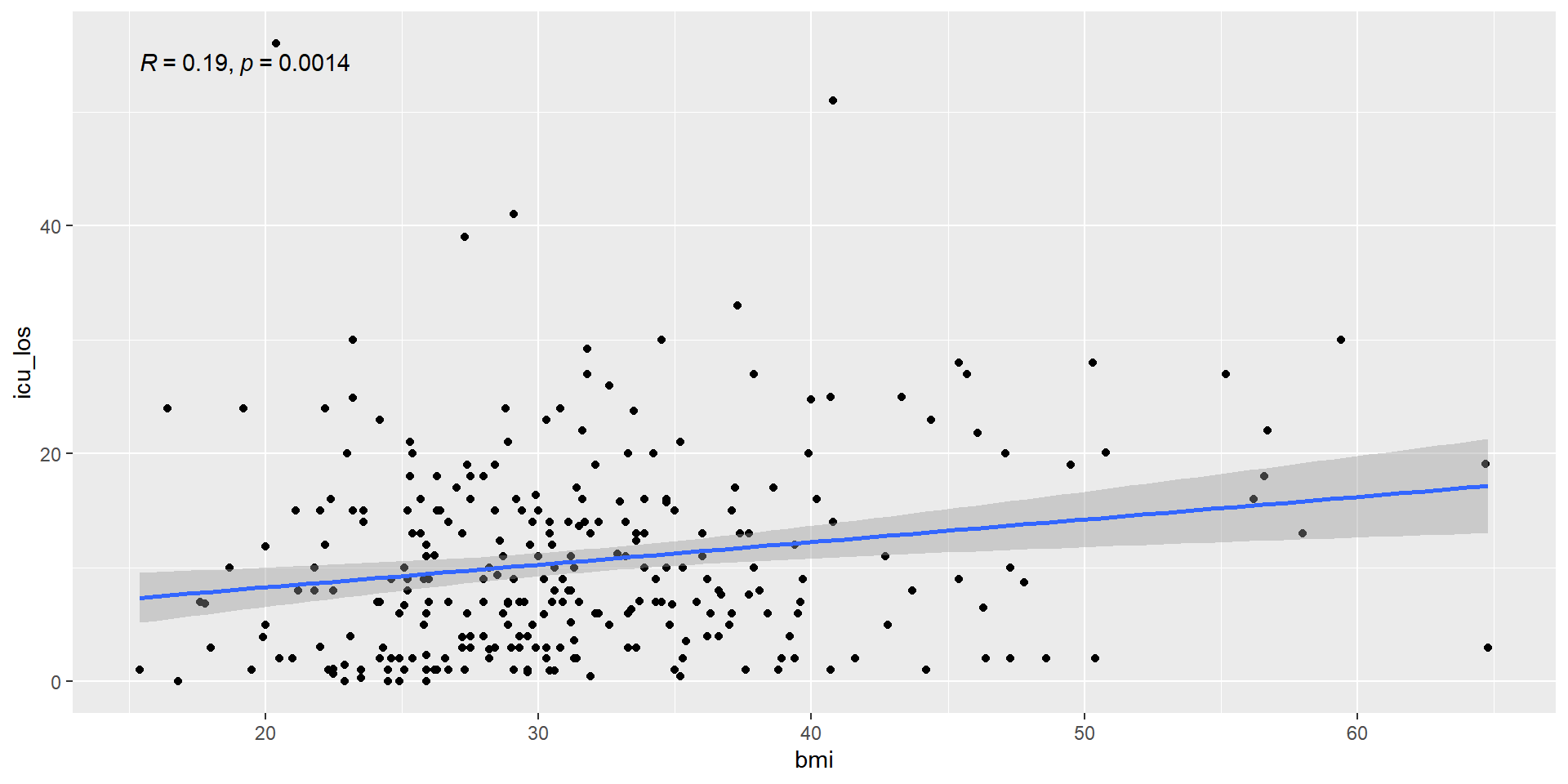
Is there a relationship between BMI and length of hospital stay in the Emory COVID dataset?
Hypothesis
\(H_0: \rho = 0\)
\(H_A: \rho \ne 0\)
Correlation Function
For correlation we will use the base R function cor.test, the cor.test function will calculate \(\rho\) and give us basic output
For correlation we must provide three arguments:
x, the first measurement continuous variabley, the second measurement continuous variableuse = "complete.obs", ignores missing values for the calculation and uses only complete observations (not sure why it doesn’t usena.rmand yes, it’s obnoxious)
Correlation Output
    Pearson's product-moment correlation

data:  qcrc_main$icu_los and qcrc_main$bmi
t = 3.234, df = 283, p-value = 0.001365
alternative hypothesis: true correlation is not equal to 0
95 percent confidence interval:
 0.07422377 0.29842419
sample estimates:
      cor
0.1887828
Correlation Output Graph Check
Always check your correlation with a graph to make sure the data is linear
Simple Linear Regression
This analysis is used to characterize the relationship between two continuous variables, where one is treated as the predictor (independent variable) and the other as the outcome (dependent variable). For example, we can analyze whether an increase in calorie intake is associated with an increase in weight. Simple linear regression provides a model to estimate this relationship using a straight-line equation.
SLR Model Equation
\(y = \beta_0 + \beta_1x + \epsilon\)
\(\beta_1\): The slope of the line, indicating the strength and direction of the relationship.
\(\beta_0\): The y-intercept, representing the value of \(y\) when \(x=0\).
\(\epsilon\): Random error.
Like correlation, regression does not imply causation! Always interpret results within the study’s context and limitations.
SLR Question
Is BMI (predictor) associated with the length of hospital stay (outcome) in the Emory COVID dataset? Meaning, if BMI changes how much (\(\beta_1\) ) does it change length of stay?
Hypothesis
\(H_0: \beta_1 = 0\)
\(H_0: \beta_1 \ne 0\)
SLR Function
We can perform simple linear regression in R using the lm() function. Here’s how the key components fit:
formula = y ~ xspecifies the dependent and independent variables.dataspecifies the dataset to use.
SLR Output
# Fit a simple linear regression model
model <- lm(icu_los ~ bmi, data = qcrc_main)

# Summarize the results
summary(model)
Call:
lm(formula = icu_los ~ bmi, data = qcrc_main)

Residuals:
    Min      1Q  Median      3Q     Max
-14.180  -6.659  -1.791   4.850  47.637

Coefficients:
            Estimate Std. Error t value Pr(>|t|)
(Intercept)   4.3119     2.0068   2.149  0.03251 *
bmi           0.1986     0.0614   3.234  0.00137 **
---
Signif. codes:  0 '***' 0.001 '**' 0.01 '*' 0.05 '.' 0.1 ' ' 1

Residual standard error: 8.625 on 283 degrees of freedom
  (3 observations deleted due to missingness)
Multiple R-squared:  0.03564,   Adjusted R-squared:  0.03223
F-statistic: 10.46 on 1 and 283 DF,  p-value: 0.001365
Output Interpretation
Estimate for \(\beta_1\): Indicates the expected change in the
icu_losfor a one-unit increase inbmi.P-value: Tests if \(\beta_1\) is significantly different from 0.
\(\mathbf{R^2}\): Proportion of variance in the outcome explained by the predictor.
Multiple Linear Regression
Multiple Linear Regression (MLR) is used to explore and model the relationship between one dependent (outcome) variable and two or more independent (predictor) variables. The goal is to understand how each predictor contributes to the outcome, while controlling for the others.
MLR Model Equation
\(y = \beta_0 + \beta_1x_1 + \beta_2x_2 + \dots + \beta_kx_k + \epsilon\)
Where:
\(y\): Dependent variable (outcome).
\(x_1, x_2, \dots, x_k\): Independent variables (predictors).
\(\beta_0\): Intercept (value of \(y\) when all \(x\)’s are 0).
\(\beta_1, \beta_2, \dots, \beta_k\): Regression coefficients, showing the change in \(y\) for a one-unit increase in \(x\), holding other variables constant.
\(\epsilon\): Random error.
MLR Question
Does BMI, age, and gender predict the length of hospital stay in the Emory COVID dataset? Or, in another way, how does length of stay change when BMI changes when we control for age and gender?
Hypothesis
\(H_0:\beta_{BMI}\;=\;\beta_{age}\;=\;\beta_{gender}\;=\;0\)
\(H_A: At\; least\; one\; \beta \neq 0\)
MLR Function
We can perform multiple linear regression in R using the lm() function. Here’s how the key components fit:
formula =\(x_1\;+\;x_2\;+\dots\;+x_k\) specifies the dependent and independent variables.dataspecifies the dataset to use.
MLR Output
# Fit the MLR model
model <- lm(icu_los ~ bmi + female + age, data = qcrc_main)

# Summarize the results
summary(model)
Call:
lm(formula = icu_los ~ bmi + female + age, data = qcrc_main)

Residuals:
    Min      1Q  Median      3Q     Max
-13.698  -6.211  -1.879   4.690  48.262

Coefficients:
            Estimate Std. Error t value Pr(>|t|)
(Intercept) -1.43801    3.69327  -0.389 0.697304
bmi          0.24431    0.06588   3.708 0.000251 ***
femaleMale   1.62934    1.02860   1.584 0.114310
age          0.05374    0.03511   1.530 0.127022
---
Signif. codes:  0 '***' 0.001 '**' 0.01 '*' 0.05 '.' 0.1 ' ' 1

Residual standard error: 8.586 on 281 degrees of freedom
  (3 observations deleted due to missingness)
Multiple R-squared:  0.05116,   Adjusted R-squared:  0.04103
F-statistic: 5.051 on 3 and 281 DF,  p-value: 0.002011
MLR Output Interpretation
Coefficients (\(\beta\)): The expected change in \(y\) for a one-unit increase in the predictor, holding all other predictors constant..
P-value: Small p-values (e.g., <0.05< 0.05<0.05) suggest a significant relationship between the predictor and the outcome.
Adjusted \(R^2\): Higher values indicate a better model fit, accounting for the number of predictors.
Logistic Regression
Logistic regression is used to model the relationship between a binary outcome variable (e.g., “died” vs. “survived”) and one or more predictor variables. It estimates the probability of the outcome occurring based on the predictors.
Logistic Model Equation
The logistic regression model predicts the log-odds of the outcome: \(\log\left(\frac{p}{1-p}\right) = \beta_0 + \beta_1 \cdot \text{female} + \beta_2 \cdot \text{intubated}\)
Where:
\(p\): Probability of the outcome occurring (e.g., \(P(died = 1)\)).
\(\beta_0\) : Intercept (log-odds of the outcome when all predictors are 0).
\(\beta_1\): Effect of being female on the log-odds of death, holding intubation status constant.
\(\beta_2\): Effect of being intubated on the log-odds of death, holding gender constant.
Logistic Question
Does gender (female) and intubation status predict the likelihood of death in the dataset?
Hypothesis
\(H_0:\beta_{female}\;=\;\beta_{intubated}\;=\;0\) (Neither gender nor intubation affect the odds of death.)
\(H_a: At\; least\; one\; \beta \neq 0\).
Logistic Function
To fit a logistic regression model in R, use the glm() function with family = binomial.
formula: Specifies the model to fit using the syntax: \(outcome \sim x_1 + x_2 +\dots+x_k\)dataspecifies the dataset to use.familySpecifies the type of regression to perform by defining the error distribution and link function. For logistic regression we usebinomialbut there are also options forgaussianandpoisson
Logistic Output
# Fit the logistic regression model
model <- glm(died ~ female + intubated, data = qcrc_main, family = binomial)

# Summarize the results
summary(model)
Call:
glm(formula = died ~ female + intubated, family = binomial, data = qcrc_main)

Coefficients:
            Estimate Std. Error z value  Pr(>|z|)
(Intercept) -1.27187    0.30248  -4.205 0.0000261 ***
femaleMale   0.05613    0.25344   0.221    0.8247
intubated    0.75926    0.31004   2.449    0.0143 *
---
Signif. codes:  0 '***' 0.001 '**' 0.01 '*' 0.05 '.' 0.1 ' ' 1

(Dispersion parameter for binomial family taken to be 1)

    Null deviance: 369.34  on 287  degrees of freedom
Residual deviance: 362.73  on 285  degrees of freedom
AIC: 368.73

Number of Fisher Scoring iterations: 4
Logistic IMPORTANT!!
The \(\beta\)s that we get from a logistic regression are useless, you MUST exponeniate them for them to be meaningful.
Logistic Output Interpretation
Example:
\(\text{Odds Ratio for Female} = \exp(0.056) \approx 1.06\): The odds of death for females are 1.06 times higher than for males.
\(\text{Odds Ratio for Intubated} = \exp(0.759) \approx 2.13\) : The odds of death for intubated patients are 2.13 times higher than for non-intubated patients.