Module 3: Iteration and vectorization in R

Learning goals

Replace repetitive code with a for loop
Use vectorization to replace unnecessary loops

Repeating code

We often want to run the same code many times, replacing just one or a few parts.

data("penguins", package = "palmerpenguins")
penguins$bill_depth_mm[penguins$island == "Biscoe"] |>
        mean(na.rm = TRUE) |>
        round(digits = 2)

[1] 15.87

penguins$bill_depth_mm[penguins$island == "Dream"] |>
        mean(na.rm = TRUE) |>
        round(digits = 2)

[1] 18.34

penguins$bill_depth_mm[penguins$island == "Torgersen"] |>
        mean(na.rm = TRUE) |>
        round(digits = 2)

[1] 18.43

We can do this ourselves if we only have a small list of changes. But imagine if there were 1000 islands instead!

What is iteration?

Whenever you repeat something, that’s iteration.
In R, this means running the same code multiple times in a row.

for (this_island in levels(penguins$island)) {
    island_mean <-
        penguins$bill_depth_mm[penguins$island == this_island] |>
        mean(na.rm = TRUE) |>
        round(digits = 2)
    
    cat(paste("The mean bill depth on", this_island, "Island was", island_mean,
                            "mm.\n"))
}

The mean bill depth on Biscoe Island was 15.87 mm.
The mean bill depth on Dream Island was 18.34 mm.
The mean bill depth on Torgersen Island was 18.43 mm.

Parts of a loop

for (this_island in levels(penguins$island)) {
    island_mean <-
        penguins$bill_depth_mm[penguins$island == this_island] |>
        mean(na.rm = TRUE) |>
        round(digits = 2)
    
    cat(paste("The mean bill depth on", this_island, "Island was", island_mean,
                            "mm.\n"))
}

The header declares how many times we will repeat the same code. The header contains a control variable that changes in each repetition and a sequence of values for the control variable to take.

Parts of a loop

for (this_island in levels(penguins$island)) {
    island_mean <-
        penguins$bill_depth_mm[penguins$island == this_island] |>
        mean(na.rm = TRUE) |>
        round(digits = 2)
    
    cat(paste("The mean bill depth on", this_island, "Island was", island_mean,
                            "mm.\n"))
}

The body of the loop contains code that will be repeated a number of times based on the header instructions. In R, the body has to be surrounded by curly braces.

Header parts

for (this_island in levels(penguins$island)) {...}

for: keyword that declares we are doing a for loop.
(...): parentheses after for declare the control variable and sequence.
this_island: the control variable.
in: keyword that separates the control varibale and sequence.
levels(penguins$island): the sequence.
{}: curly braces will contain the body code.

Header parts

for (this_island in levels(penguins$island)) {...}

Since levels(penguins$island) evaluates to c("Biscoe", "Dream", "Torgersen"), our loop will repeat 3 times.

Iteration	`this_island`
1	“Biscoe”
2	“Dream”
3	“Torgersen”

Everything inside of {...} will be repeated three times.

Loop iteration 1

island_mean <-
    penguins$bill_depth_mm[penguins$island == "Biscoe"] |>
    mean(na.rm = TRUE) |>
    round(digits = 2)

cat(paste("The mean bill depth on", "Biscoe", "Island was", island_mean,
                    "mm.\n"))

The mean bill depth on Biscoe Island was 15.87 mm.

Loop iteration 2

island_mean <-
    penguins$bill_depth_mm[penguins$island == "Dream"] |>
    mean(na.rm = TRUE) |>
    round(digits = 2)

cat(paste("The mean bill depth on", "Dream", "Island was", island_mean,
                    "mm.\n"))

The mean bill depth on Dream Island was 18.34 mm.

Loop iteration 3

island_mean <-
    penguins$bill_depth_mm[penguins$island == "Torgersen"] |>
    mean(na.rm = TRUE) |>
    round(digits = 2)

cat(paste("The mean bill depth on", "Torgersen", "Island was", island_mean,
                    "mm.\n"))

The mean bill depth on Torgersen Island was 18.43 mm.

The loop structure automates this process for us so we don’t have to copy and paste our code!

for (this_island in levels(penguins$island)) {
    island_mean <-
        penguins$bill_depth_mm[penguins$island == this_island] |>
        mean(na.rm = TRUE) |>
        round(digits = 2)
    
    cat(paste("The mean bill depth on", this_island, "Island was", island_mean,
                            "mm.\n"))
}

The mean bill depth on Biscoe Island was 15.87 mm.
The mean bill depth on Dream Island was 18.34 mm.
The mean bill depth on Torgersen Island was 18.43 mm.

Side note: the pipe operator `|>`

This operator allows us to chain commands together so the output of the previous statement is passed into the next statement.
E.g. the code

island_mean <-
    penguins$bill_depth_mm[penguins$island == "Torgersen"] |>
    mean(na.rm = TRUE) |>
    round(digits = 2)

will be transformed by R into

island_mean <-
    round(
        mean(
            penguins$bill_depth_mm[penguins$island == "Torgersen"],
            na.rm = TRUE
        ),
        digits = 2
    )

before it gets run. So using the pipe is a way to avoid deeply nested functions.

Note that another alernative could be like this:

island_data <- penguins$bill_depth_mm[penguins$island == "Torgersen"]
island_mean_raw <- mean(island_data, na.rm = TRUE)
island_mean <- round(island_mean_raw, digits = 2)

So using |> can also help us to avoid a lot of assignments.

Whichever style you prefer is fine! Some people like the pipe, some people like nesting, and some people like intermediate assignments. All three are perfectly fine as long as your code is neat and commented.
If you go on to the tidyverse class, you will use a lot of piping – it is a very popular coding style in R these days thanks to the inventors of the tidyverse packages.
Also note that you need R version 4.1.0 or better to use |>. If you are on an older version of R, it will not be available.

Now, back to loops!

Remember: write DRY code!

DRY = “Don’t Repeat Yourself”
Instead of copying and pasting, write loops and functions.
Easier to debug and change in the future!

Of course, we all copy and paste code sometimes. If you are running on a tight deadline or can’t get a loop or function to work, you might need to. DRY code is good, but working code is best!

You try it!

Write a loop that goes from 1 to 10, squares each of the numbers, and prints the squared number.

for (i in 1:10) {
    cat(i ^ 2, "\n")
}

Wait, did we need to do that?

Well, yes, because you need to practice loops!
But technically no, because we can use vectorization.
Almost all basic operations in R are vectorized: they work on a vector of arguments all at the same time.

Wait, did we need to do that?

Well, yes, because you need to practice loops!
But technically no, because we can use vectorization.
Almost all basic operations in R are vectorized: they work on a vector of arguments all at the same time.
(Technical note: actually, vectorized operations still do a loop. But they do the loop inside a compiled C program, which is much faster than R loops.)

# No loop needed!
(1:10)^2

 [1]   1   4   9  16  25  36  49  64  81 100

# Get the first 10 odd numbers, a common CS 101 loop problem on exams
(1:20)[which((1:20 %% 2) == 1)]

 [1]  1  3  5  7  9 11 13 15 17 19

So you should really try vectorization first, then use loops only when you can’t use vectorization.

Loop walkthrough

Let’s walk through a complex but useful example where we can’t use vectorization.
Load the cleaned measles dataset, and subset it so you only have MCV1 records.

meas <- readRDS(here::here("data", "measles_final.Rds"))
str(meas)

spc_tbl_ [9,416 × 9] (S3: spec_tbl_df/tbl_df/tbl/data.frame)
 $ iso3c        : chr [1:9416] "AFG" "AFG" "AFG" "AFG" ...
 $ year         : num [1:9416] 2023 2022 2021 2020 2019 ...
 $ measles_cases: num [1:9416] 2792 5166 2900 640 353 ...
 $ population   : num [1:9416] 42239854 41128771 40099462 38972230 37769499 ...
 $ MCV1_coverage: num [1:9416] NA 68 63 66 64 71 67 64 62 60 ...
 $ MCV2_coverage: num [1:9416] NA 49 44 43 41 49 40 40 42 44 ...
 $ country      : chr [1:9416] "Afghanistan" "Afghanistan" "Afghanistan" "Afghanistan" ...
 $ region       : chr [1:9416] "Asia" "Asia" "Asia" "Asia" ...
 $ sub_region   : chr [1:9416] "Southern Asia" "Southern Asia" "Southern Asia" "Southern Asia" ...
 - attr(*, "spec")=List of 3
  ..$ cols   :List of 6
  .. ..$ iso3c        : list()
  .. .. ..- attr(*, "class")= chr [1:2] "collector_character" "collector"
  .. ..$ year         : list()
  .. .. ..- attr(*, "class")= chr [1:2] "collector_double" "collector"
  .. ..$ measles_cases: list()
  .. .. ..- attr(*, "class")= chr [1:2] "collector_double" "collector"
  .. ..$ population   : list()
  .. .. ..- attr(*, "class")= chr [1:2] "collector_double" "collector"
  .. ..$ MCV1_coverage: list()
  .. .. ..- attr(*, "class")= chr [1:2] "collector_double" "collector"
  .. ..$ MCV2_coverage: list()
  .. .. ..- attr(*, "class")= chr [1:2] "collector_double" "collector"
  ..$ default: list()
  .. ..- attr(*, "class")= chr [1:2] "collector_guess" "collector"
  ..$ delim  : chr ","
  ..- attr(*, "class")= chr "col_spec"
 - attr(*, "problems")=<externalptr>

Loop walkthrough

First, make an empty list. This is where we’ll store our results. Make it the same length as the number of countries in the dataset.

res <- vector(mode = "list", length = length(unique(meas$country)))

This is called preallocation and it can make your loops much faster.

Loop walkthrough

Loop through every country in the dataset, and get the median, first and third quartiles, and range for each country. Store those summary statistics in a data frame.
What should the header look like?

countries <- unique(meas$country)
for (i in 1:length(countries)) {...}

Note that we use the index as the control variable. When you need to do complex operations inside a loop, this is easier than the for-each construction we used earlier.

Loop walkthrough

Now write out the body of the code. First we need to subset the data, to get only the data for the current country.

for (i in 1:length(countries)) {
    # Get the data for the current country only
    country_data <- subset(meas, country == countries[i])
}

Next we need to get the summary of the cases for that country.

for (i in 1:length(countries)) {
    # Get the data for the current country only
    country_data <- subset(meas, country == countries[i])
    
    # Get the summary statistics for this country
    country_cases <- country_data$measles_cases
    country_quart <- quantile(
        country_cases, na.rm = TRUE, probs = c(0.25, 0.5, 0.75)
    )
    country_range <- range(country_cases, na.rm = TRUE)
}

Next we save the summary statistics into a data frame.

for (i in 1:length(countries)) {
    # Get the data for the current country only
    country_data <- subset(meas, country == countries[i])
    
    # Get the summary statistics for this country
    country_cases <- country_data$measles_cases
    country_quart <- quantile(
        country_cases, na.rm = TRUE, probs = c(0.25, 0.5, 0.75)
    )
    country_range <- range(country_cases, na.rm = TRUE)
    
    # Save the summary statistics into a data frame
    country_summary <- data.frame(
        country = countries[[i]],
        min = country_range[[1]],
        Q1 = country_quart[[1]],
        median = country_quart[[2]],
        Q3 = country_quart[[3]],
        max = country_range[[2]]
    )
}

And finally, we save the data frame as the next element in our storage list.

for (i in 1:length(countries)) {
    # Get the data for the current country only
    country_data <- subset(meas, country == countries[i])
    
    # Get the summary statistics for this country
    country_cases <- country_data$measles_cases
    country_quart <- quantile(
        country_cases, na.rm = TRUE, probs = c(0.25, 0.5, 0.75)
    )
    country_range <- range(country_cases, na.rm = TRUE)
    
    # Save the summary statistics into a data frame
    country_summary <- data.frame(
        country = countries[[i]],
        min = country_range[[1]],
        Q1 = country_quart[[1]],
        median = country_quart[[2]],
        Q3 = country_quart[[3]],
        max = country_range[[2]]
    )
    
    # Save the results to our container
    res[[i]] <- country_summary
}

Warning in min(x): no non-missing arguments to min; returning Inf

Warning in max(x): no non-missing arguments to max; returning -Inf

Let’s take a look at the results.

head(res)

[[1]]
      country min   Q1 median     Q3   max
1 Afghanistan 353 1158 2345.5 6190.5 32455

[[2]]
  country min Q1 median Q3    max
1 Albania   0  1     12 29 136034

[[3]]
  country min  Q1 median   Q3   max
1 Algeria   0 112   2686 8204 29584

[[4]]
         country min Q1 median  Q3 max
1 American Samoa   0  0      0 2.5 498

[[5]]
  country min Q1 median Q3 max
1 Andorra   0  0      0  0   5

[[6]]
  country min    Q1 median    Q3   max
1  Angola  29 732.5 3389.5 15878 30067

How do we deal with this to get it into a nice form?

We can use a vectorization trick: the function do.call() seems like ancient computer science magic. And it is. But it will actually help us a lot.

res_df <- do.call(rbind, res)
head(res_df)

country	min	Q1	median	Q3	max
Afghanistan	353	1158.0	2345.5	6190.5	32455
Albania	0	1.0	12.0	29.0	136034
Algeria	0	112.0	2686.0	8204.0	29584
American Samoa	0	0.0	0.0	2.5	498
Andorra	0	0.0	0.0	0.0	5
Angola	29	732.5	3389.5	15878.0	30067

It combined our data frames together! Let’s take a look at the rbind and do.call() help packages to see what happened.

?rbind

Combine R Objects by Rows or Columns

Description:

     Take a sequence of vector, matrix or data-frame arguments and
     combine by _c_olumns or _r_ows, respectively.  These are generic
     functions with methods for other R classes.

Usage:

     cbind(..., deparse.level = 1)
     rbind(..., deparse.level = 1)
     ## S3 method for class 'data.frame'
     rbind(..., deparse.level = 1, make.row.names = TRUE,
           stringsAsFactors = FALSE, factor.exclude = TRUE)
     
Arguments:

     ...: (generalized) vectors or matrices.  These can be given as
          named arguments.  Other R objects may be coerced as
          appropriate, or S4 methods may be used: see sections
          'Details' and 'Value'.  (For the '"data.frame"' method of
          'cbind' these can be further arguments to 'data.frame' such
          as 'stringsAsFactors'.)

deparse.level: integer controlling the construction of labels in the
          case of non-matrix-like arguments (for the default method):
          'deparse.level = 0' constructs no labels;
          the default 'deparse.level = 1' typically and 'deparse.level
          = 2' always construct labels from the argument names, see the
          'Value' section below.

make.row.names: (only for data frame method:) logical indicating if
          unique and valid 'row.names' should be constructed from the
          arguments.

stringsAsFactors: logical, passed to 'as.data.frame'; only has an
          effect when the '...' arguments contain a (non-'data.frame')
          'character'.

factor.exclude: if the data frames contain factors, the default 'TRUE'
          ensures that 'NA' levels of factors are kept, see PR#17562
          and the 'Data frame methods'.  In R versions up to 3.6.x,
          'factor.exclude = NA' has been implicitly hardcoded (R <=
          3.6.0) or the default (R = 3.6.x, x >= 1).

Details:

     The functions 'cbind' and 'rbind' are S3 generic, with methods for
     data frames.  The data frame method will be used if at least one
     argument is a data frame and the rest are vectors or matrices.
     There can be other methods; in particular, there is one for time
     series objects.  See the section on 'Dispatch' for how the method
     to be used is selected.  If some of the arguments are of an S4
     class, i.e., 'isS4(.)' is true, S4 methods are sought also, and
     the hidden 'cbind' / 'rbind' functions from package 'methods'
     maybe called, which in turn build on 'cbind2' or 'rbind2',
     respectively.  In that case, 'deparse.level' is obeyed, similarly
     to the default method.

     In the default method, all the vectors/matrices must be atomic
     (see 'vector') or lists.  Expressions are not allowed.  Language
     objects (such as formulae and calls) and pairlists will be coerced
     to lists: other objects (such as names and external pointers) will
     be included as elements in a list result.  Any classes the inputs
     might have are discarded (in particular, factors are replaced by
     their internal codes).

     If there are several matrix arguments, they must all have the same
     number of columns (or rows) and this will be the number of columns
     (or rows) of the result.  If all the arguments are vectors, the
     number of columns (rows) in the result is equal to the length of
     the longest vector.  Values in shorter arguments are recycled to
     achieve this length (with a 'warning' if they are recycled only
     _fractionally_).

     When the arguments consist of a mix of matrices and vectors the
     number of columns (rows) of the result is determined by the number
     of columns (rows) of the matrix arguments.  Any vectors have their
     values recycled or subsetted to achieve this length.

     For 'cbind' ('rbind'), vectors of zero length (including 'NULL')
     are ignored unless the result would have zero rows (columns), for
     S compatibility.  (Zero-extent matrices do not occur in S3 and are
     not ignored in R.)

     Matrices are restricted to less than 2^31 rows and columns even on
     64-bit systems.  So input vectors have the same length
     restriction: as from R 3.2.0 input matrices with more elements
     (but meeting the row and column restrictions) are allowed.

Value:

     For the default method, a matrix combining the '...' arguments
     column-wise or row-wise.  (Exception: if there are no inputs or
     all the inputs are 'NULL', the value is 'NULL'.)

     The type of a matrix result determined from the highest type of
     any of the inputs in the hierarchy raw < logical < integer <
     double < complex < character < list .

     For 'cbind' ('rbind') the column (row) names are taken from the
     'colnames' ('rownames') of the arguments if these are matrix-like.
     Otherwise from the names of the arguments or where those are not
     supplied and 'deparse.level > 0', by deparsing the expressions
     given, for 'deparse.level = 1' only if that gives a sensible name
     (a 'symbol', see 'is.symbol').

     For 'cbind' row names are taken from the first argument with
     appropriate names: rownames for a matrix, or names for a vector of
     length the number of rows of the result.

     For 'rbind' column names are taken from the first argument with
     appropriate names: colnames for a matrix, or names for a vector of
     length the number of columns of the result.

Data frame methods:

     The 'cbind' data frame method is just a wrapper for
     'data.frame(..., check.names = FALSE)'.  This means that it will
     split matrix columns in data frame arguments.

     The 'rbind' data frame method first drops all zero-column and
     zero-row arguments.  (If that leaves none, it returns the first
     argument with columns otherwise a zero-column zero-row data
     frame.)  It then takes the classes of the columns from the first
     data frame, and matches columns by name (rather than by position).
     Factors have their levels expanded as necessary (in the order of
     the levels of the level sets of the factors encountered) and the
     result is an ordered factor if and only if all the components were
     ordered factors.  Old-style categories (integer vectors with
     levels) are promoted to factors.

     Note that for result column 'j', 'factor(., exclude = X(j))' is
     applied, where

       X(j) := if(isTRUE(factor.exclude)) {
                  if(!NA.lev[j]) NA # else NULL
               } else factor.exclude
     
     where 'NA.lev[j]' is true iff any contributing data frame has had
     a 'factor' in column 'j' with an explicit 'NA' level.

Dispatch:

     The method dispatching is _not_ done via 'UseMethod()', but by
     C-internal dispatching.  Therefore there is no need for, e.g.,
     'rbind.default'.

     The dispatch algorithm is described in the source file
     ('.../src/main/bind.c') as

       1. For each argument we get the list of possible class
          memberships from the class attribute.

       2. We inspect each class in turn to see if there is an
          applicable method.

       3. If we find a method, we use it.  Otherwise, if there was an
          S4 object among the arguments, we try S4 dispatch; otherwise,
          we use the default code.

     If you want to combine other objects with data frames, it may be
     necessary to coerce them to data frames first.  (Note that this
     algorithm can result in calling the data frame method if all the
     arguments are either data frames or vectors, and this will result
     in the coercion of character vectors to factors.)

References:

     Becker, R. A., Chambers, J. M. and Wilks, A. R. (1988) _The New S
     Language_.  Wadsworth & Brooks/Cole.

See Also:

     'c' to combine vectors (and lists) as vectors, 'data.frame' to
     combine vectors and matrices as a data frame.

Examples:

     m <- cbind(1, 1:7) # the '1' (= shorter vector) is recycled
     m
     m <- cbind(m, 8:14)[, c(1, 3, 2)] # insert a column
     m
     cbind(1:7, diag(3)) # vector is subset -> warning
     
     cbind(0, rbind(1, 1:3))
     cbind(I = 0, X = rbind(a = 1, b = 1:3))  # use some names
     xx <- data.frame(I = rep(0,2))
     cbind(xx, X = rbind(a = 1, b = 1:3))   # named differently
     
     cbind(0, matrix(1, nrow = 0, ncol = 4)) #> Warning (making sense)
     dim(cbind(0, matrix(1, nrow = 2, ncol = 0))) #-> 2 x 1
     
     ## deparse.level
     dd <- 10
     rbind(1:4, c = 2, "a++" = 10, dd, deparse.level = 0) # middle 2 rownames
     rbind(1:4, c = 2, "a++" = 10, dd, deparse.level = 1) # 3 rownames (default)
     rbind(1:4, c = 2, "a++" = 10, dd, deparse.level = 2) # 4 rownames
     
     ## cheap row names:
     b0 <- gl(3,4, labels=letters[1:3])
     bf <- setNames(b0, paste0("o", seq_along(b0)))
     df  <- data.frame(a = 1, B = b0, f = gl(4,3))
     df. <- data.frame(a = 1, B = bf, f = gl(4,3))
     new <- data.frame(a = 8, B ="B", f = "1")
     (df1  <- rbind(df , new))
     (df.1 <- rbind(df., new))
     stopifnot(identical(df1, rbind(df,  new, make.row.names=FALSE)),
               identical(df1, rbind(df., new, make.row.names=FALSE)))

?do.call

Execute a Function Call

Description:

     'do.call' constructs and executes a function call from a name or a
     function and a list of arguments to be passed to it.

Usage:

     do.call(what, args, quote = FALSE, envir = parent.frame())
     
Arguments:

    what: either a function or a non-empty character string naming the
          function to be called.

    args: a _list_ of arguments to the function call.  The 'names'
          attribute of 'args' gives the argument names.

   quote: a logical value indicating whether to quote the arguments.

   envir: an environment within which to evaluate the call.  This will
          be most useful if 'what' is a character string and the
          arguments are symbols or quoted expressions.

Details:

     If 'quote' is 'FALSE', the default, then the arguments are
     evaluated (in the calling environment, not in 'envir').  If
     'quote' is 'TRUE' then each argument is quoted (see 'quote') so
     that the effect of argument evaluation is to remove the quotes -
     leaving the original arguments unevaluated when the call is
     constructed.

     The behavior of some functions, such as 'substitute', will not be
     the same for functions evaluated using 'do.call' as if they were
     evaluated from the interpreter.  The precise semantics are
     currently undefined and subject to change.

Value:

     The result of the (evaluated) function call.

Warning:

     This should not be used to attempt to evade restrictions on the
     use of '.Internal' and other non-API calls.

References:

     Becker, R. A., Chambers, J. M. and Wilks, A. R. (1988) _The New S
     Language_.  Wadsworth & Brooks/Cole.

See Also:

     'call' which creates an unevaluated call.

Examples:

     do.call("complex", list(imaginary = 1:3))
     
     ## if we already have a list (e.g., a data frame)
     ## we need c() to add further arguments
     tmp <- expand.grid(letters[1:2], 1:3, c("+", "-"))
     do.call("paste", c(tmp, sep = ""))
     
     do.call(paste, list(as.name("A"), as.name("B")), quote = TRUE)
     
     ## examples of where objects will be found.
     A <- 2
     f <- function(x) print(x^2)
     env <- new.env()
     assign("A", 10, envir = env)
     assign("f", f, envir = env)
     f <- function(x) print(x)
     f(A)                                      # 2
     do.call("f", list(A))                     # 2
     do.call("f", list(A), envir = env)        # 4
     do.call( f,  list(A), envir = env)        # 2
     do.call("f", list(quote(A)), envir = env) # 100
     do.call( f,  list(quote(A)), envir = env) # 10
     do.call("f", list(as.name("A")), envir = env) # 100
     
     eval(call("f", A))                      # 2
     eval(call("f", quote(A)))               # 2
     eval(call("f", A), envir = env)         # 4
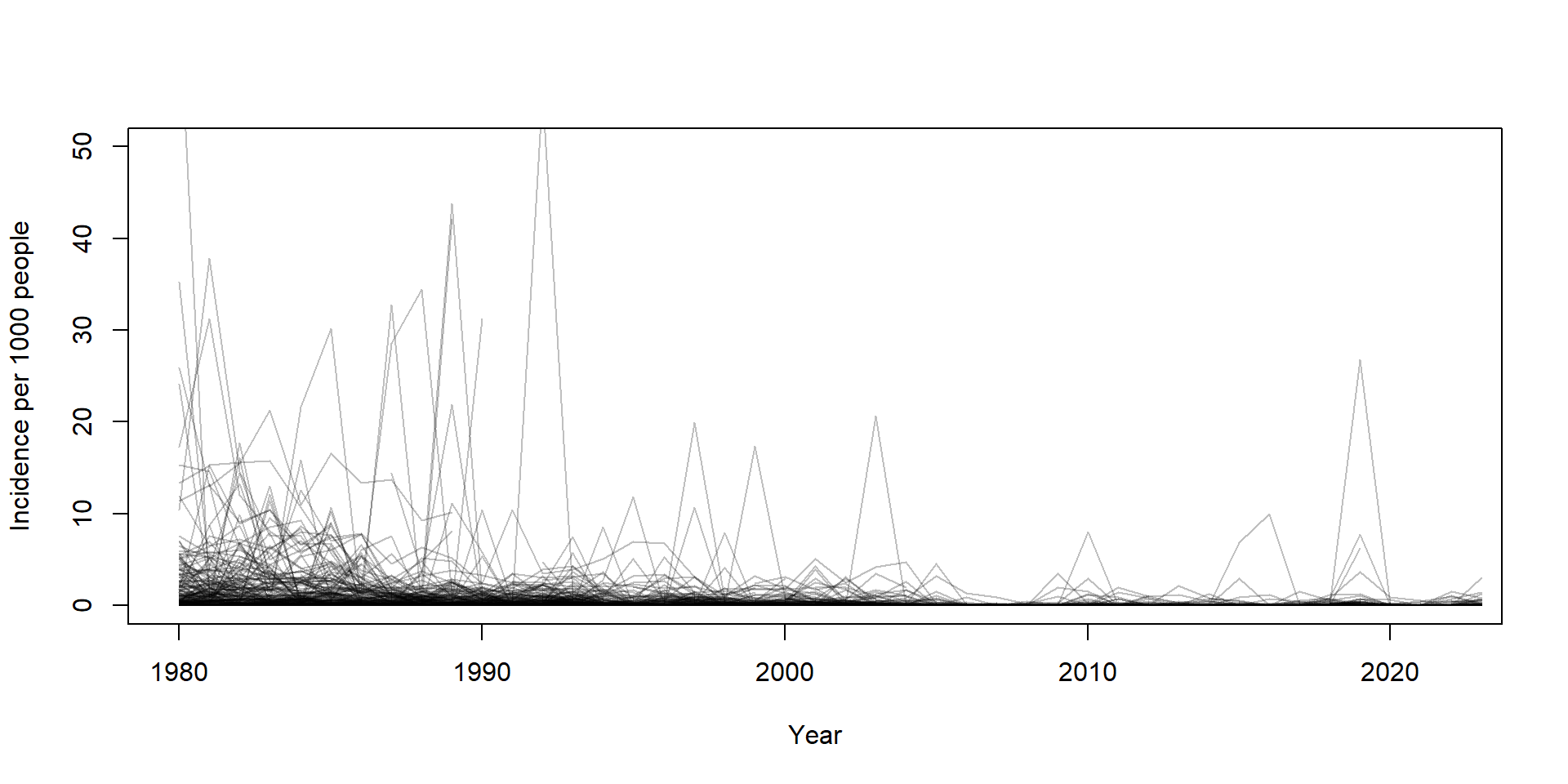
     eval(call("f", quote(A)), envir = env)  # 100

OK, so basically what happened is that

do.call(rbind, list)

Gets transformed into

rbind(list[[1]], list[[2]], list[[3]], ..., list[[length(list)]])

That’s vectorization magic!

You try it! (if we have time)

Use the code you wrote before the get the incidence per 1000 people on the entire measles data set (add a column for incidence to the full data).
Use the code plot(NULL, NULL, ...) to make a blank plot. You will need to set the xlim and ylim arguments to sensible values, and specify the axis titles as “Year” and “Incidence per 1000 people”.
Using a for loop and the lines() function, make a plot that shows all of the incidence curves over time, overlapping on the plot.
HINT: use col = adjustcolor(black, alpha.f = 0.25) to make the curves partially transparent, so you can see the overlap.
BONUS PROBLEM: using the function cumsum(), make a plot of the cumulative cases (not standardized) over time for all of the countries. (Dealing with the NA’s here is tricky!!)

Main problem hint

meas$cases_per_thousand <- meas$measles_cases / meas$population * 1000
countries <- unique(meas$country)

plot(
    NULL, NULL,
    xlim = c(1980, 2022),
    ylim = c(0, 50),
    xlab = "Year",
    ylab = "Incidence per 1000 people"
)

for (...) {
    ...
}

Main problem solution

meas$cases_per_thousand <- meas$measles_cases / meas$population * 1000
countries <- unique(meas$country)

plot(
    NULL, NULL,
    xlim = c(1980, 2022),
    ylim = c(0, 50),
    xlab = "Year",
    ylab = "Incidence per 1000 people"
)

for (i in 1:length(countries)) {
    country_data <- subset(meas, country == countries[[i]])
    lines(
        x = country_data$year,
        y = country_data$cases_per_thousand,
        col = adjustcolor("black", alpha.f = 0.25)
    )
}

Main problem solution

Bonus problem solution

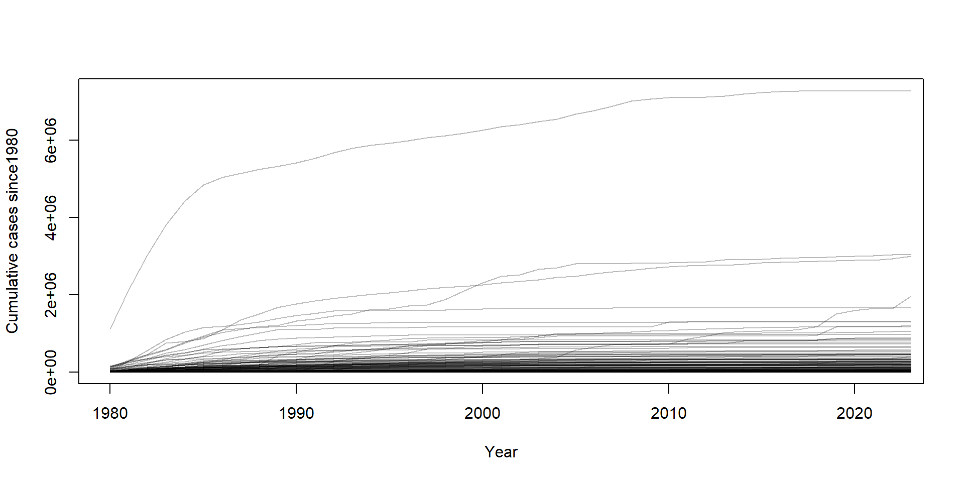
# First calculate the cumulative cases, treating NA as zeroes
meas2 <- dplyr::arrange(meas, iso3c, year)
meas2$cumulative_cases <- ave(
    x = ifelse(is.na(meas2$measles_cases), 0, meas2$measles_cases),
    meas2$country,
    FUN = cumsum
)

plot(
    NULL, NULL,
    xlim = c(1980, 2022),
    ylim = c(1, 7.3e6),
    xlab = "Year",
    ylab = paste0("Cumulative cases since", min(meas2$year))
)

for (i in 1:length(countries)) {
    country_data <- subset(meas2, country == countries[[i]])
    lines(
        x = country_data$year,
        y = country_data$cumulative_cases,
        col = adjustcolor("black", alpha.f = 0.25)
    )
}

Module 3: Iteration and vectorization in R

Learning goals

Repeating code

What is iteration?

Parts of a loop

Parts of a loop

Header parts

Header parts

Loop iteration 1

Loop iteration 2

Loop iteration 3

The loop structure automates this process for us so we don’t have to copy and paste our code!

Side note: the pipe operator |>

Remember: write DRY code!

You try it!

Wait, did we need to do that?

Wait, did we need to do that?

Loop walkthrough

Loop walkthrough

Loop walkthrough

Loop walkthrough

You try it! (if we have time)

Main problem hint

Main problem solution

Main problem solution

Bonus problem solution

Bonus problem solution

Side note: the pipe operator `|>`