Object Summaries

Description:

     'summary' is a generic function used to produce result summaries
     of the results of various model fitting functions.  The function
     invokes particular 'methods' which depend on the 'class' of the
     first argument.

Usage:

     summary(object, ...)

     ## Default S3 method:
     summary(object, ..., digits, quantile.type = 7)
     ## S3 method for class 'data.frame'
     summary(object, maxsum = 7,
            digits = max(3, getOption("digits")-3), ...)

     ## S3 method for class 'factor'
     summary(object, maxsum = 100, ...)

     ## S3 method for class 'matrix'
     summary(object, ...)

     ## S3 method for class 'summaryDefault'
     format(x, digits = max(3L, getOption("digits") - 3L), zdigits = 4L, ...)
      ## S3 method for class 'summaryDefault'
     print(x, digits = max(3L, getOption("digits") - 3L), zdigits = 4L, ...)

Arguments:

  object: an object for which a summary is desired.

       x: a result of the _default_ method of 'summary()'.

  maxsum: integer, indicating how many levels should be shown for
          'factor's.

  digits: integer (or 'NULL', see 'Details'), used for number
          formatting with 'signif()' (for 'summary.default') or
          'format()' (for 'summary.data.frame').  In 'summary.default',
          if not specified (i.e., 'missing(.)'), 'signif()' will _not_
          be called anymore (since R >= 3.4.0, where the default has
          been changed to only round in the 'print' and 'format'
          methods).

 zdigits: integer, typically positive to be used in the internal
          'zapsmall(*, digits = digits + zdigits)' call.

quantile.type: integer code used in 'quantile(*, type=quantile.type)'
          for the default method.

     ...: additional arguments affecting the summary produced.

Details:

     For 'factor's, the frequency of the first 'maxsum - 1' most
     frequent levels is shown, and the less frequent levels are
     summarized in '"(Others)"' (resulting in at most 'maxsum'
     frequencies).

     The 'digits' argument may be 'NULL' for some methods specifying to
     use the default value, e.g., for the '"summaryDefault"' 'format()'
     method.

     The functions 'summary.lm' and 'summary.glm' are examples of
     particular methods which summarize the results produced by 'lm'
     and 'glm'.

Value:

     The form of the value returned by 'summary' depends on the class
     of its argument.  See the documentation of the particular methods
     for details of what is produced by that method.

     The default method returns an object of class 'c("summaryDefault",
     "table")' which has specialized 'format' and 'print' methods.  The
     'factor' method returns an integer vector.

     The matrix and data frame methods return a matrix of class
     '"table"', obtained by applying 'summary' to each column and
     collating the results.

References:

     Chambers, J. M. and Hastie, T. J. (1992) _Statistical Models in
     S_.  Wadsworth & Brooks/Cole.

See Also:

     'anova', 'summary.glm', 'summary.lm'.

Examples:

     summary(attenu, digits = 4) #-> summary.data.frame(...), default precision
     summary(attenu $ station, maxsum = 20) #-> summary.factor(...)

     lst <- unclass(attenu$station) > 20 # logical with NAs
     ## summary.default() for logicals -- different from *.factor:
     summary(lst)
     summary(as.factor(lst))

     ## show the effect of zdigits for skewed data
     set.seed(17); x <- rlnorm(100, sdlog=2)
     dput(sx <- summary(x))
     sx # exponential format for this data
print(sx, zdigits = 3) # fixed point: "more readable"Module 6: S3 and R Formulas
Learning goals
- Explain what S3 is and give an example of an S3 method
- Understand the R help pages for S3 methods
- Use vectorization to replace unnecessary loops
- Understand when and how to use the R formula syntax
- Write basic linear models with R formulas
Part 1: S3 stands for 3/10 Scariness
Objects and classes and methods
- We’ve talked about imperative programming and functional programming. Now we’ll talk about object-oriented programming.
- S3 is a “functional OOP” system, which is different from OOP you might have dealt with in Python or C++.
- The main propery of S3 is polymorphism: one generic function can act differently on different classes of objects, but symbolically represents the same thing and has a consistent interface.
An S3 example
summary()is an example of an S3 generic. And the documentation tells us this.
Polymorphism of summary
- When we call
summary(an_object)it determines what it should do based on the class ofan_object. - Each of the following summaries shows us different statistics.
[1] "lm"
Call:
lm(formula = bwt ~ age, data = birthwt)

Residuals:
     Min       1Q   Median       3Q      Max
-2294.78  -517.63    10.51   530.80  1774.92

Coefficients:
            Estimate Std. Error t value Pr(>|t|)
(Intercept)  2655.74     238.86   11.12   <2e-16 ***
age            12.43      10.02    1.24    0.216
---
Signif. codes:  0 '***' 0.001 '**' 0.01 '*' 0.05 '.' 0.1 ' ' 1

Residual standard error: 728.2 on 187 degrees of freedom
Multiple R-squared:  0.008157,  Adjusted R-squared:  0.002853
F-statistic: 1.538 on 1 and 187 DF, p-value: 0.2165[1] "glm" "lm"
Call:
glm(formula = low ~ age, family = "binomial", data = birthwt)

Coefficients:
            Estimate Std. Error z value Pr(>|z|)
(Intercept)  0.38458    0.73212   0.525    0.599
age         -0.05115    0.03151  -1.623    0.105

(Dispersion parameter for binomial family taken to be 1)

    Null deviance: 234.67  on 188  degrees of freedom
Residual deviance: 231.91  on 187  degrees of freedom
AIC: 235.91

Number of Fisher Scoring iterations: 4[1] "glmerMod"
attr(,"package")
[1] "lme4"Generalized linear mixed model fit by maximum likelihood (Laplace
Approximation) [glmerMod]
Family: binomial ( logit )
Formula: low ~ age + (1 | id)
Data: birthwt
AIC BIC logLik -2*log(L) df.resid
237.9 247.6 -116.0 231.9 186
Scaled residuals:
Min 1Q Median 3Q Max
-0.8451 -0.7066 -0.5908 1.3042 1.9639
Random effects:
Groups Name Variance Std.Dev.
id (Intercept) 0.009912 0.09956
Number of obs: 189, groups: id, 189
Fixed effects:
Estimate Std. Error z value Pr(>|z|)
(Intercept) 0.38540 0.73534 0.524 0.600
age -0.05127 0.03234 -1.585 0.113
Correlation of Fixed Effects:
(Intr)
age -0.966Some OOP definitions
- A class is a category of object. Objects of the same class have the same fields or attributes.
- A generic is a function that has different behavior for multiple classes of inputs.
- The methods for a function are the function implementations for specific classes.
- Method dispatch is the process where you call a generic function, the generic function checks the class of the input, and the generic function calls the method for that class.
- A default method is dispatched by a generic function when there is no specific method for the class of the input. Not every generic has a default method.
S3 classes
- Everything that exists in R is an object and has a type.
- But not everything is an S3 object, and only S3 objects have a class.
- This is confusing, because the function
class()will tell you something for every object, no matter what. If an object does not have a class,class()will return the type. - To check if an object has an S3 class, you have to check the extremely confusing
attr(an_object, "class")instead.
S3 classes (and types)
- These objects have types but not classes:
NULL, vectors, lists, functions, and some other special ones that you won’t use. - You can pretty much pretend that types are classes.
S3 classes (and types)
S3 classes (and types)
S3 classes (and types)
- If an object has an S3 class, then it is a list.
- The only things that aren’t lists are the other special objects with types.
- Complicated S3 classes are just lists where the elements have specific names.
List of 12
 $ coefficients : Named num [1:2] 2655.7 12.4
  ..- attr(*, "names")= chr [1:2] "(Intercept)" "age"
 $ residuals    : Named num [1:189] -369 -515 -347 -323 -279 ...
  ..- attr(*, "names")= chr [1:189] "85" "86" "87" "88" ...
 $ effects      : Named num [1:189] -40481 -903 -340 -309 -284 ...
  ..- attr(*, "names")= chr [1:189] "(Intercept)" "age" "" "" ...
 $ rank         : int 2
 $ fitted.values: Named num [1:189] 2892 3066 2904 2917 2879 ...
  ..- attr(*, "names")= chr [1:189] "85" "86" "87" "88" ...
 $ assign       : int [1:2] 0 1
 $ qr           :List of 5
  ..$ qr   : num [1:189, 1:2] -13.7477 0.0727 0.0727 0.0727 0.0727 ...
  .. ..- attr(*, "dimnames")=List of 2
  .. .. ..$ : chr [1:189] "85" "86" "87" "88" ...
  .. .. ..$ : chr [1:2] "(Intercept)" "age"
  .. ..- attr(*, "assign")= int [1:2] 0 1
  ..$ qraux: num [1:2] 1.07 1.14
  ..$ pivot: int [1:2] 1 2
  ..$ tol  : num 1e-07
  ..$ rank : int 2
  ..- attr(*, "class")= chr "qr"
 $ df.residual  : int 187
 $ xlevels      : Named list()
 $ call         : language lm(formula = bwt ~ age, data = birthwt)
 $ terms        :Classes 'terms', 'formula'  language bwt ~ age
  .. ..- attr(*, "variables")= language list(bwt, age)
  .. ..- attr(*, "factors")= int [1:2, 1] 0 1
  .. .. ..- attr(*, "dimnames")=List of 2
  .. .. .. ..$ : chr [1:2] "bwt" "age"
  .. .. .. ..$ : chr "age"
  .. ..- attr(*, "term.labels")= chr "age"
  .. ..- attr(*, "order")= int 1
  .. ..- attr(*, "intercept")= int 1
  .. ..- attr(*, "response")= int 1
  .. ..- attr(*, ".Environment")=<environment: R_GlobalEnv>
  .. ..- attr(*, "predvars")= language list(bwt, age)
  .. ..- attr(*, "dataClasses")= Named chr [1:2] "numeric" "numeric"
  .. .. ..- attr(*, "names")= chr [1:2] "bwt" "age"
 $ model        :'data.frame':  189 obs. of  2 variables:
  ..$ bwt: int [1:189] 2523 2551 2557 2594 2600 2622 2637 2637 2663 2665 ...
  ..$ age: int [1:189] 19 33 20 21 18 21 22 17 29 26 ...
  ..- attr(*, "terms")=Classes 'terms', 'formula'  language bwt ~ age
  .. .. ..- attr(*, "variables")= language list(bwt, age)
  .. .. ..- attr(*, "factors")= int [1:2, 1] 0 1
  .. .. .. ..- attr(*, "dimnames")=List of 2
  .. .. .. .. ..$ : chr [1:2] "bwt" "age"
  .. .. .. .. ..$ : chr "age"
  .. .. ..- attr(*, "term.labels")= chr "age"
  .. .. ..- attr(*, "order")= int 1
  .. .. ..- attr(*, "intercept")= int 1
  .. .. ..- attr(*, "response")= int 1
  .. .. ..- attr(*, ".Environment")=<environment: R_GlobalEnv>
  .. .. ..- attr(*, "predvars")= language list(bwt, age)
  .. .. ..- attr(*, "dataClasses")= Named chr [1:2] "numeric" "numeric"
  .. .. .. ..- attr(*, "names")= chr [1:2] "bwt" "age"
- attr(*, "class")= chr "lm"Fitting Linear Models
Description:
'lm' is used to fit linear models, including multivariate ones.
It can be used to carry out regression, single stratum analysis of
variance and analysis of covariance (although 'aov' may provide a
more convenient interface for these).
Usage:
lm(formula, data, subset, weights, na.action,
method = "qr", model = TRUE, x = FALSE, y = FALSE, qr = TRUE,
singular.ok = TRUE, contrasts = NULL, offset, ...)
## S3 method for class 'lm'
print(x, digits = max(3L, getOption("digits") - 3L), ...)
Arguments:
formula: an object of class '"formula"' (or one that can be coerced to
that class): a symbolic description of the model to be
fitted. The details of model specification are given under
'Details'.
data: an optional data frame, list or environment (or object
coercible by 'as.data.frame' to a data frame) containing the
variables in the model. If not found in 'data', the
variables are taken from 'environment(formula)', typically
the environment from which 'lm' is called.
subset: an optional vector specifying a subset of observations to be
used in the fitting process. (See additional details about
how this argument interacts with data-dependent bases in the
'Details' section of the 'model.frame' documentation.)
weights: an optional vector of weights to be used in the fitting
process. Should be 'NULL' or a numeric vector. If non-NULL,
weighted least squares is used with weights 'weights' (that
is, minimizing 'sum(w*e^2)'); otherwise ordinary least
squares is used. See also 'Details',
na.action: a function which indicates what should happen when the data
contain 'NA's. The default is set by the 'na.action' setting
of 'options', and is 'na.fail' if that is unset. The
'factory-fresh' default is 'na.omit'. Another possible value
is 'NULL', no action. Value 'na.exclude' can be useful.
method: the method to be used; for fitting, currently only 'method =
"qr"' is supported; 'method = "model.frame"' returns the
model frame (the same as with 'model = TRUE', see below).
model, x, y, qr: logicals. If 'TRUE' the corresponding components of
the fit (the model frame, the model matrix, the response, the
QR decomposition) are returned.
singular.ok: logical. If 'FALSE' (the default in S but not in R) a
singular fit is an error.
contrasts: an optional list. See the 'contrasts.arg' of
'model.matrix.default'.
offset: this can be used to specify an _a priori_ known component to
be included in the linear predictor during fitting. This
should be 'NULL' or a numeric vector or matrix of extents
matching those of the response. One or more 'offset' terms
can be included in the formula instead or as well, and if
more than one are specified their sum is used. See
'model.offset'.
...: For 'lm()': additional arguments to be passed to the low
level regression fitting functions (see below).
digits: the number of _significant_ digits to be passed to
'format(coef(x), .)' when 'print()'ing.
Details:
Models for 'lm' are specified symbolically. A typical model has
the form 'response ~ terms' where 'response' is the (numeric)
response vector and 'terms' is a series of terms which specifies a
linear predictor for 'response'. A terms specification of the
form 'first + second' indicates all the terms in 'first' together
with all the terms in 'second' with duplicates removed. A
specification of the form 'first:second' indicates the set of
terms obtained by taking the interactions of all terms in 'first'
with all terms in 'second'. The specification 'first*second'
indicates the _cross_ of 'first' and 'second'. This is the same
as 'first + second + first:second'.
If the formula includes an 'offset', this is evaluated and
subtracted from the response.
If 'response' is a matrix a linear model is fitted separately by
least-squares to each column of the matrix and the result inherits
from '"mlm"' ("multivariate linear model").
See 'model.matrix' for some further details. The terms in the
formula will be re-ordered so that main effects come first,
followed by the interactions, all second-order, all third-order
and so on: to avoid this pass a 'terms' object as the formula (see
'aov' and 'demo(glm.vr)' for an example).
A formula has an implied intercept term. To remove this use
either 'y ~ x - 1' or 'y ~ 0 + x'. See 'formula' for more details
of allowed formulae.
Non-'NULL' 'weights' can be used to indicate that different
observations have different variances (with the values in
'weights' being inversely proportional to the variances); or
equivalently, when the elements of 'weights' are positive integers
w_i, that each response y_i is the mean of w_i unit-weight
observations (including the case that there are w_i observations
equal to y_i and the data have been summarized). However, in the
latter case, notice that within-group variation is not used.
Therefore, the sigma estimate and residual degrees of freedom may
be suboptimal; in the case of replication weights, even wrong.
Hence, standard errors and analysis of variance tables should be
treated with care.
'lm' calls the lower level functions 'lm.fit', etc, see below, for
the actual numerical computations. For programming only, you may
consider doing likewise.
All of 'weights', 'subset' and 'offset' are evaluated in the same
way as variables in 'formula', that is first in 'data' and then in
the environment of 'formula'.
Value:
'lm' returns an object of 'class' '"lm"' or for multivariate
('multiple') responses of class 'c("mlm", "lm")'.
The functions 'summary' and 'anova' are used to obtain and print a
summary and analysis of variance table of the results. The
generic accessor functions 'coefficients', 'effects',
'fitted.values' and 'residuals' extract various useful features of
the value returned by 'lm'.
An object of class '"lm"' is a list containing at least the
following components:
coefficients: a named vector of coefficients
residuals: the residuals, that is response minus fitted values.
fitted.values: the fitted mean values.
rank: the numeric rank of the fitted linear model.
weights: (only for weighted fits) the specified weights.
df.residual: the residual degrees of freedom.
call: the matched call.
terms: the 'terms' object used.
contrasts: (only where relevant) the contrasts used.
xlevels: (only where relevant) a record of the levels of the factors
used in fitting.
offset: the offset used (missing if none were used).
y: if requested, the response used.
x: if requested, the model matrix used.
model: if requested (the default), the model frame used.
na.action: (where relevant) information returned by 'model.frame' on
the special handling of 'NA's.
In addition, non-null fits will have components 'assign',
'effects' and (unless not requested) 'qr' relating to the linear
fit, for use by extractor functions such as 'summary' and
'effects'.
Using time series:
Considerable care is needed when using 'lm' with time series.
Unless 'na.action = NULL', the time series attributes are stripped
from the variables before the regression is done. (This is
necessary as omitting 'NA's would invalidate the time series
attributes, and if 'NA's are omitted in the middle of the series
the result would no longer be a regular time series.)
Even if the time series attributes are retained, they are not used
to line up series, so that the time shift of a lagged or
differenced regressor would be ignored. It is good practice to
prepare a 'data' argument by 'ts.intersect(..., dframe = TRUE)',
then apply a suitable 'na.action' to that data frame and call 'lm'
with 'na.action = NULL' so that residuals and fitted values are
time series.
Author(s):
The design was inspired by the S function of the same name
described in Chambers (1992). The implementation of model formula
by Ross Ihaka was based on Wilkinson & Rogers (1973).
References:
Chambers, J. M. (1992) _Linear models._ Chapter 4 of _Statistical
Models in S_ eds J. M. Chambers and T. J. Hastie, Wadsworth &
Brooks/Cole.
Wilkinson, G. N. and Rogers, C. E. (1973). Symbolic descriptions
of factorial models for analysis of variance. _Applied
Statistics_, *22*, 392-399. doi:10.2307/2346786
<https://doi.org/10.2307/2346786>.
See Also:
'summary.lm' for more detailed summaries and 'anova.lm' for the
ANOVA table; 'aov' for a different interface.
The generic functions 'coef', 'effects', 'residuals', 'fitted',
'vcov'.
'predict.lm' (via 'predict') for prediction, including confidence
and prediction intervals; 'confint' for confidence intervals of
_parameters_.
'lm.influence' for regression diagnostics, and 'glm' for
*generalized* linear models.
The underlying low level functions, 'lm.fit' for plain, and
'lm.wfit' for weighted regression fitting.
More 'lm()' examples are available e.g., in 'anscombe',
'attitude', 'freeny', 'LifeCycleSavings', 'longley', 'stackloss',
'swiss'.
'biglm' in package 'biglm' for an alternative way to fit linear
models to large datasets (especially those with many cases).
Examples:
require(graphics)
## Annette Dobson (1990) "An Introduction to Generalized Linear Models".
## Page 9: Plant Weight Data.
ctl <- c(4.17,5.58,5.18,6.11,4.50,4.61,5.17,4.53,5.33,5.14)
trt <- c(4.81,4.17,4.41,3.59,5.87,3.83,6.03,4.89,4.32,4.69)
group <- gl(2, 10, 20, labels = c("Ctl","Trt"))
weight <- c(ctl, trt)
lm.D9 <- lm(weight ~ group)
lm.D90 <- lm(weight ~ group - 1) # omitting intercept
anova(lm.D9)
summary(lm.D90)
opar <- par(mfrow = c(2,2), oma = c(0, 0, 1.1, 0))
plot(lm.D9, las = 1) # Residuals, Fitted, ...
par(opar)
### less simple examples in "See Also" aboveS3 help pages
- Now you know enough to understand the help pages for S3 objects.
Object Summaries

Description:

     'summary' is a generic function used to produce result summaries
     of the results of various model fitting functions.  The function
     invokes particular 'methods' which depend on the 'class' of the
     first argument.

Usage:

     summary(object, ...)

     ## Default S3 method:
     summary(object, ..., digits, quantile.type = 7)
     ## S3 method for class 'data.frame'
     summary(object, maxsum = 7,
            digits = max(3, getOption("digits")-3), ...)

     ## S3 method for class 'factor'
     summary(object, maxsum = 100, ...)

     ## S3 method for class 'matrix'
     summary(object, ...)

     ## S3 method for class 'summaryDefault'
     format(x, digits = max(3L, getOption("digits") - 3L), zdigits = 4L, ...)
      ## S3 method for class 'summaryDefault'
     print(x, digits = max(3L, getOption("digits") - 3L), zdigits = 4L, ...)

Arguments:

  object: an object for which a summary is desired.

       x: a result of the _default_ method of 'summary()'.

  maxsum: integer, indicating how many levels should be shown for
          'factor's.

  digits: integer (or 'NULL', see 'Details'), used for number
          formatting with 'signif()' (for 'summary.default') or
          'format()' (for 'summary.data.frame').  In 'summary.default',
          if not specified (i.e., 'missing(.)'), 'signif()' will _not_
          be called anymore (since R >= 3.4.0, where the default has
          been changed to only round in the 'print' and 'format'
          methods).

 zdigits: integer, typically positive to be used in the internal
          'zapsmall(*, digits = digits + zdigits)' call.

quantile.type: integer code used in 'quantile(*, type=quantile.type)'
          for the default method.

     ...: additional arguments affecting the summary produced.

Details:

     For 'factor's, the frequency of the first 'maxsum - 1' most
     frequent levels is shown, and the less frequent levels are
     summarized in '"(Others)"' (resulting in at most 'maxsum'
     frequencies).

     The 'digits' argument may be 'NULL' for some methods specifying to
     use the default value, e.g., for the '"summaryDefault"' 'format()'
     method.

     The functions 'summary.lm' and 'summary.glm' are examples of
     particular methods which summarize the results produced by 'lm'
     and 'glm'.

Value:

     The form of the value returned by 'summary' depends on the class
     of its argument.  See the documentation of the particular methods
     for details of what is produced by that method.

     The default method returns an object of class 'c("summaryDefault",
     "table")' which has specialized 'format' and 'print' methods.  The
     'factor' method returns an integer vector.

     The matrix and data frame methods return a matrix of class
     '"table"', obtained by applying 'summary' to each column and
     collating the results.

References:

     Chambers, J. M. and Hastie, T. J. (1992) _Statistical Models in
     S_.  Wadsworth & Brooks/Cole.

See Also:

     'anova', 'summary.glm', 'summary.lm'.

Examples:

     summary(attenu, digits = 4) #-> summary.data.frame(...), default precision
     summary(attenu $ station, maxsum = 20) #-> summary.factor(...)

     lst <- unclass(attenu$station) > 20 # logical with NAs
     ## summary.default() for logicals -- different from *.factor:
     summary(lst)
     summary(as.factor(lst))

     ## show the effect of zdigits for skewed data
     set.seed(17); x <- rlnorm(100, sdlog=2)
     dput(sx <- summary(x))
     sx # exponential format for this data
     print(sx, zdigits = 3) # fixed point: "more readable"
Finding classes and finding methods
- Use the
methods()function to find all methods that are available for a specific generic function.
 [1] summary,ANY-method                  summary,diagonalMatrix-method
 [3] summary,sparseMatrix-method         summary.allFit*
 [5] summary.aov                         summary.aovlist*
 [7] summary.aspell*                     summary.check_packages_in_dir*
 [9] summary.connection                  summary.corAR1*
[11] summary.corARMA*                    summary.corCAR1*
[13] summary.corCompSymm*                summary.corExp*
[15] summary.corGaus*                    summary.corIdent*
[17] summary.corLin*                     summary.corNatural*
[19] summary.corRatio*                   summary.corSpher*
[21] summary.corStruct*                  summary.corSymm*
[23] summary.data.frame                  summary.Date
[25] summary.default                     summary.difftime
[27] summary.ecdf*                       summary.factor
[29] summary.glm                         summary.gls*
[31] summary.infl*                       summary.lm
[33] summary.lme*                        summary.lmList*
[35] summary.lmList4*                    summary.loess*
[37] summary.loglm*                      summary.manova
[39] summary.matrix                      summary.merMod*
[41] summary.mlm*                        summary.modelStruct*
[43] summary.negbin*                     summary.nls*
[45] summary.nlsList*                    summary.packageStatus*
[47] summary.pdBlocked*                  summary.pdCompSymm*
[49] summary.pdDiag*                     summary.pdIdent*
[51] summary.pdLogChol*                  summary.pdMat*
[53] summary.pdNatural*                  summary.pdSymm*
[55] summary.polr*                       summary.POSIXct
[57] summary.POSIXlt                     summary.ppr*
[59] summary.prcomp*                     summary.prcomplist*
[61] summary.princomp*                   summary.proc_time
[63] summary.reStruct*                   summary.rlang:::list_of_conditions*
[65] summary.rlang_error*                summary.rlang_message*
[67] summary.rlang_trace*                summary.rlang_warning*
[69] summary.rlm*                        summary.shingle*
[71] summary.srcfile                     summary.srcref
[73] summary.stepfun                     summary.stl*
[75] summary.summary.merMod*             summary.table
[77] summary.trellis*                    summary.tukeysmooth*
[79] summary.varComb*                    summary.varConstPower*
[81] summary.varConstProp*               summary.varExp*
[83] summary.varFixed*                   summary.varFunc*
[85] summary.varIdent*                   summary.varPower*
[87] summary.warnings
see '?methods' for accessing help and source code- Also use the
methods(class = ...)function to find all methods that are available for a specific class.
 [1] add1           alias          anova          case.names     coerce
 [6] confint        cooks.distance deviance       dfbeta         dfbetas
[11] drop1          dummy.coef     effects        extractAIC     family
[16] formula        hatvalues      influence      initialize     kappa
[21] labels         logLik         model.frame    model.matrix   nobs
[26] plot           predict        print          proj           qqnorm
[31] qr             residuals      rstandard      rstudent       show
[36] simulate       slotsFromS3    summary        variable.names vcov
see '?methods' for accessing help and source code- You can use a dot (
.) to reference specific methods, not just generics.
Summarizing Linear Model Fits

Description:

     'summary' method for class '"lm"'.

Usage:

     ## S3 method for class 'lm'
     summary(object, correlation = FALSE, symbolic.cor = FALSE, ...)

     ## S3 method for class 'summary.lm'
     print(x, digits = max(3, getOption("digits") - 3),
           symbolic.cor = x$symbolic.cor,
           signif.stars = getOption("show.signif.stars"), ...)

Arguments:

  object: an object of class '"lm"', usually, a result of a call to
          'lm'.

       x: an object of class '"summary.lm"', usually, a result of a
          call to 'summary.lm'.

correlation: logical; if 'TRUE', the correlation matrix of the
          estimated parameters is returned and printed.

  digits: the number of significant digits to use when printing.

symbolic.cor: logical. If 'TRUE', print the correlations in a symbolic
          form (see 'symnum') rather than as numbers.

signif.stars: logical. If 'TRUE', 'significance stars' are printed for
          each coefficient.

     ...: further arguments passed to or from other methods.

Details:

     'print.summary.lm' tries to be smart about formatting the
     coefficients, standard errors, etc. and additionally gives
     'significance stars' if 'signif.stars' is 'TRUE'.

     Aliased coefficients are omitted in the returned object but
     restored by the 'print' method.

     Correlations are printed to two decimal places (or symbolically):
     to see the actual correlations print 'summary(object)$correlation'
     directly.

Value:

     The function 'summary.lm' computes and returns a list of summary
     statistics of the fitted linear model given in 'object', using the
     components (list elements) '"call"' and '"terms"' from its
     argument, plus

residuals: the _weighted_ residuals, the usual residuals rescaled by
          the square root of the weights specified in the call to 'lm'.

coefficients: a p x 4 matrix with columns for the estimated
          coefficient, its standard error, t-statistic and
          corresponding (two-sided) p-value.  Aliased coefficients are
          omitted.

 aliased: named logical vector showing if the original coefficients are
          aliased.

   sigma: the square root of the estimated variance of the random error

                       sigma^2 = 1/(n-p) Sum(w[i] R[i]^2),

          where R[i] is the i-th residual, 'residuals[i]'.

      df: degrees of freedom, a 3-vector (p, n-p, p*), the first being
          the number of non-aliased coefficients, the last being the
          total number of coefficients.

fstatistic: (for models including non-intercept terms) a 3-vector with
          the value of the F-statistic with its numerator and
          denominator degrees of freedom.

r.squared: R^2, the 'fraction of variance explained by the model',

                    R^2 = 1 - Sum(R[i]^2) / Sum((y[i]- y*)^2),

          where y* is the mean of y[i] if there is an intercept and
          zero otherwise.

adj.r.squared: the above R^2 statistic '_adjusted_', penalizing for
          higher p.

cov.unscaled: a p x p matrix of (unscaled) covariances of the coef[j],
          j=1, ..., p.

correlation: the correlation matrix corresponding to the above
          'cov.unscaled', if 'correlation = TRUE' is specified.

symbolic.cor: (only if 'correlation' is true.)  The value of the
          argument 'symbolic.cor'.

na.action: from 'object', if present there.

See Also:

     The model fitting function 'lm', 'summary'.

     Function 'coef' will extract the matrix of coefficients with
     standard errors, t-statistics and p-values.

Examples:

     ##-- Continuing the  lm(.) example:
     coef(lm.D90)  # the bare coefficients
     sld90 <- summary(lm.D90 <- lm(weight ~ group -1))  # omitting intercept
     sld90
     coef(sld90)  # much more

     ## model with *aliased* coefficient:
     lm.D9. <- lm(weight ~ group + I(group != "Ctl"))
     Sm.D9. <- summary(lm.D9.)
     Sm.D9. #  shows the NA NA NA NA  line
     stopifnot(length(cc <- coef(lm.D9.)) == 3, is.na(cc[3]),
               dim(coef(Sm.D9.)) == c(2,4), Sm.D9.$df == c(2, 18, 3))
Part 2: Formulas / Formulae
Utility of S3 methods
- Hopefully you can now see why understanding S3 methods is important.
- But if you aren’t convinced, maybe
formulaobjects can convince you. Look how many methods there are!
 [1] [             aggregate     alias         all.equal     ansari.test
 [6] barplot       bartlett.test boxplot       cdplot        coerce
[11] cor.test      deriv         deriv3        fligner.test  formula
[16] friedman.test ftable        getInitial    head          initialize
[21] kruskal.test  ks.test       lines         mood.test     mosaicplot
[26] pairs         plot          points        ppr           prcomp
[31] princomp      print         quade.test    selfStart     show
[36] simulate      slotsFromS3   spineplot     stripchart    sunflowerplot
[41] t.test        terms         text          update        var.test
[46] wilcox.test
see '?methods' for accessing help and source code- And that doesn’t include functions like
lm()which ONLY have methods for formulas, not generics.
Formula example
- Say you want to get the correlation between MCV1 coverage rate and measles cases in Pakistan. You can call the
cor.test()function by passing two vectors.
meas <- readr::read_rds(here::here("data", "measles_final.Rds"))

cor.test(
    x = meas$MCV1_coverage[meas$iso3c == "PAK"],
    y = meas$measles_cases[meas$iso3c == "PAK"]
)
    Pearson's product-moment correlation

data:  meas$MCV1_coverage[meas$iso3c == "PAK"] and meas$measles_cases[meas$iso3c == "PAK"]
t = -3.2036, df = 41, p-value = 0.002627
alternative hypothesis: true correlation is not equal to 0
95 percent confidence interval:
 -0.6591955 -0.1699300
sample estimates:
       cor
-0.4474377 - But if we inspect the methods for
cor.test, we see it is an S3 generic with a method forformulaclass objects.
- Typing in the code is easier, and reading the output is easier.
    Pearson's product-moment correlation

data:  measles_cases and MCV1_coverage
t = -3.2036, df = 41, p-value = 0.002627
alternative hypothesis: true correlation is not equal to 0
95 percent confidence interval:
 -0.6591955 -0.1699300
sample estimates:
       cor
-0.4474377 - But it pays to understand S3, because in certain circumstances, using the default method is easier!
Writing formulas
- The formula language is a smaller language inside of R used for writing statistical models, and the full details are in the
?formuladocumentation. - This little formula language is so useful it is now used in many textbooks and other languages (Python and Julia).
- The basic syntax is
dv ~ iv1 + iv2 + .... - Recall that in
cor.test()our formula didn’t have a LHS – there is no dependent variable in correlation.
You try it!
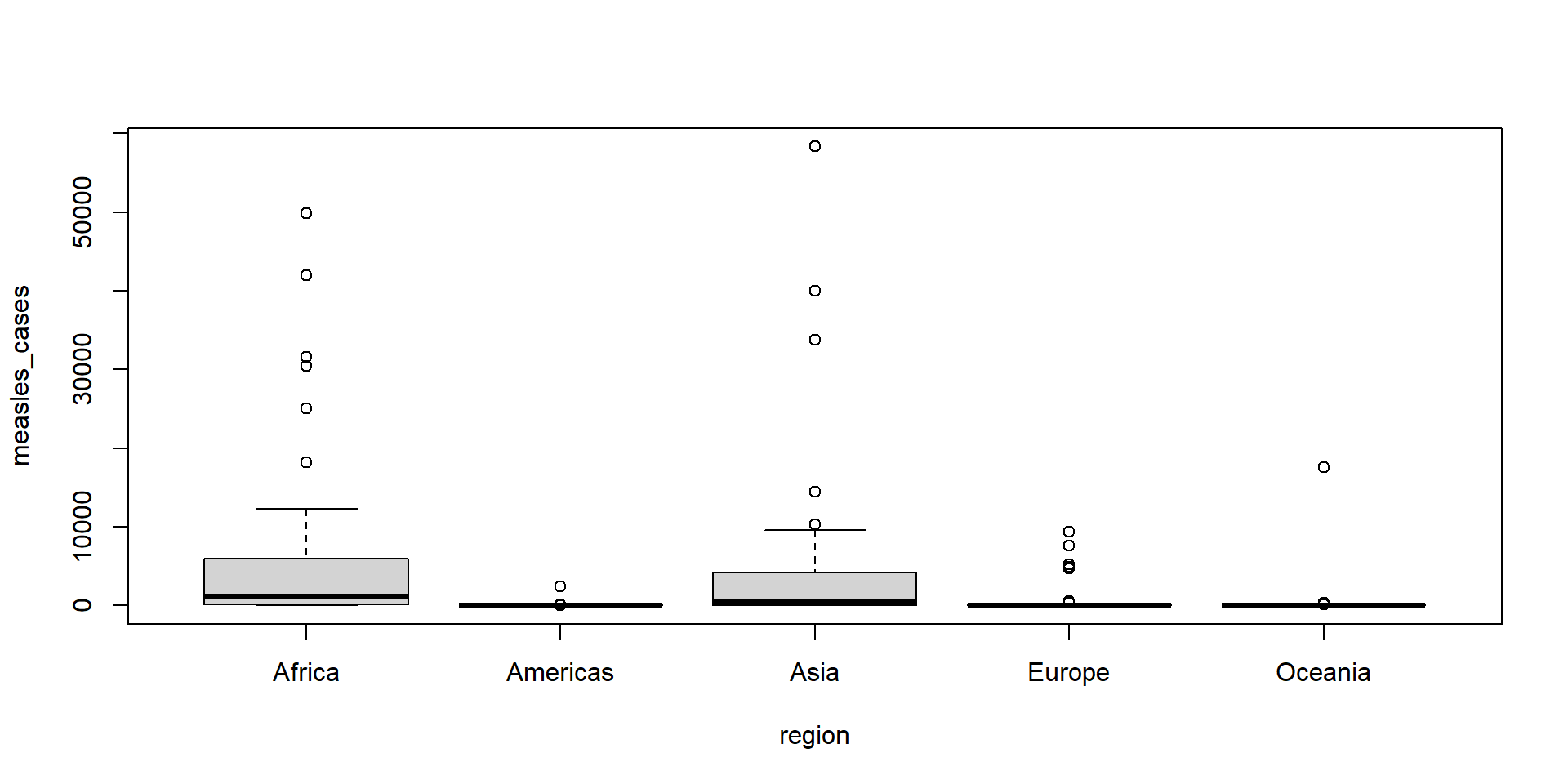
- Before, we saw that
boxplothad a formula method. Useboxplot()with a formula to make boxplots of measles cases in 2002 for eachregionin the dataset.
- Hint: your code should look like this for the correct DV and IV.
You try it (more advanced)
- Load the QCRC dataset, you only need the sheet “Main_Dataset” for this.
- Fit a logistic regression model with 30 day mortality (
30D_Mortalityin the spreadsheet) as the outcome. Include any continuous or categorical predictors you want, we recommend avoiding variables that are (supposed to be) date/times. - Use appropriate S3 generic functions to get statistics about your model that you would want to report.
- Hint: to read in the data, do this.
- Hint: you might need to do some data cleaning, because missing data are written as a period in the spreadsheet.
- Hint: your logistic regression code should look like this.
- Hint: you need to put backticks (this thing: `, NOT an apostrophe. It’s made by the ~ key on american keyboards.) around the name of the variable `30D_Mortality`.
- Hint: some useful functions with methods for
glm-class objects aresummary,coef, andconfint. (You probably also need the functionexp!)
- One solution, you could have used any predictors you want, though you should be able to explain why they might affect 30 Day mortality.
# A little cleaning for D Dimer
# First turn the "." into actual NA's and make it a real number
qcrc$d_dimer <- as.numeric(dplyr::na_if(qcrc$`D dimer`, "."))
# Take the log cause it's skewed and positive
qcrc$d_dimer <- log(qcrc$d_dimer)
# Impute missing values with the median -- there are much better ways to do this
med_d_dimer <- median(qcrc$d_dimer, na.rm = FALSE)
qcrc$d_dimer <- ifelse(is.na(qcrc$d_dimer), med_d_dimer, qcrc$d_dimer)

# A little cleaning for Race
qcrc$Race <- factor(qcrc$Race) |>
    # Make White the reference level
    relevel(ref = "Caucasian or White") |>
    # Groups other than "Causian or White" and "Black or African American" are
    # really small and heterogeneous so put them together
    # Not ideal but sometimes the best we can do
    forcats::fct_lump_n(n = 2)

# Fit a model that controls for treatment, d_dimer, and race/ethnicity
model_30dm <- glm(
    `30D_Mortality` ~ Remdesivir_or_placebo + d_dimer + Race,
    data = qcrc,
    family = "binomial"
)- Look at a lot of useful information with
summary().
Call:
glm(formula = `30D_Mortality` ~ Remdesivir_or_placebo + d_dimer +
    Race, family = "binomial", data = qcrc)

Coefficients:
                               Estimate Std. Error z value Pr(>|z|)
(Intercept)                     -2.4352     0.8190  -2.973  0.00295 **
Remdesivir_or_placebo           -0.7004     0.4105  -1.706  0.08793 .
d_dimer                          0.1848     0.1015   1.820  0.06871 .
RaceAfrican American  or Black   0.2738     0.3899   0.702  0.48260
RaceOther                        0.7733     0.4990   1.550  0.12119
---
Signif. codes:  0 '***' 0.001 '**' 0.01 '*' 0.05 '.' 0.1 ' ' 1

(Dispersion parameter for binomial family taken to be 1)

    Null deviance: 317.14  on 256  degrees of freedom
Residual deviance: 308.52  on 252  degrees of freedom
  (31 observations deleted due to missingness)
AIC: 318.52

Number of Fisher Scoring iterations: 4- Get the OR’s with
coef().
- Get the profile CI’s with
confint().
- A basic interpretation of the coefficient for
Remdesivir_or_placebo(coded as 1 for remdesivir and 0 for placebo) might be “Odds of mortality after 30 days in the remdesivisir group were 0.48 times the odds in the placebo group, for patients with the same D dimer level and race/ethnicity. The 95% CI for the odds ratio was 0.20 to 1.04. The effect was not significant at the \(\alpha = 0.05\) significance group, but is suggestive that at least some patients benefitted from remdesivir treatment.”
Summary
- We learned the basics of “functional OOP” and specifically R’s S3 system, including how to check classes and find S3 methods for a class or classes for an S3 method.
- We learned the basics of R formulas, a consistent and powerful sub-language in R for writing statistical models.
- There’s a lot more to formulas, but we’ll discuss them more in a separate module based on interest/time.
- If you want to read more about S3 or OOP in R, check out the OOP section in Wickham’s Advanced R.