Module XX: FP Applications
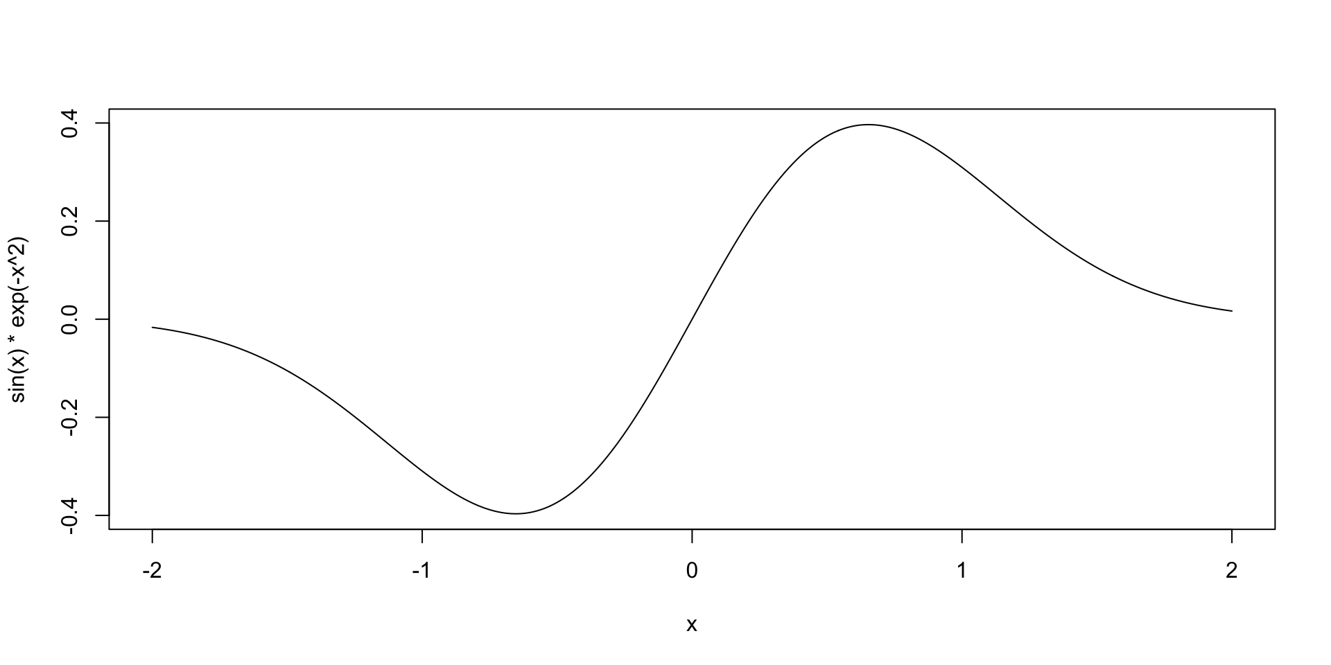
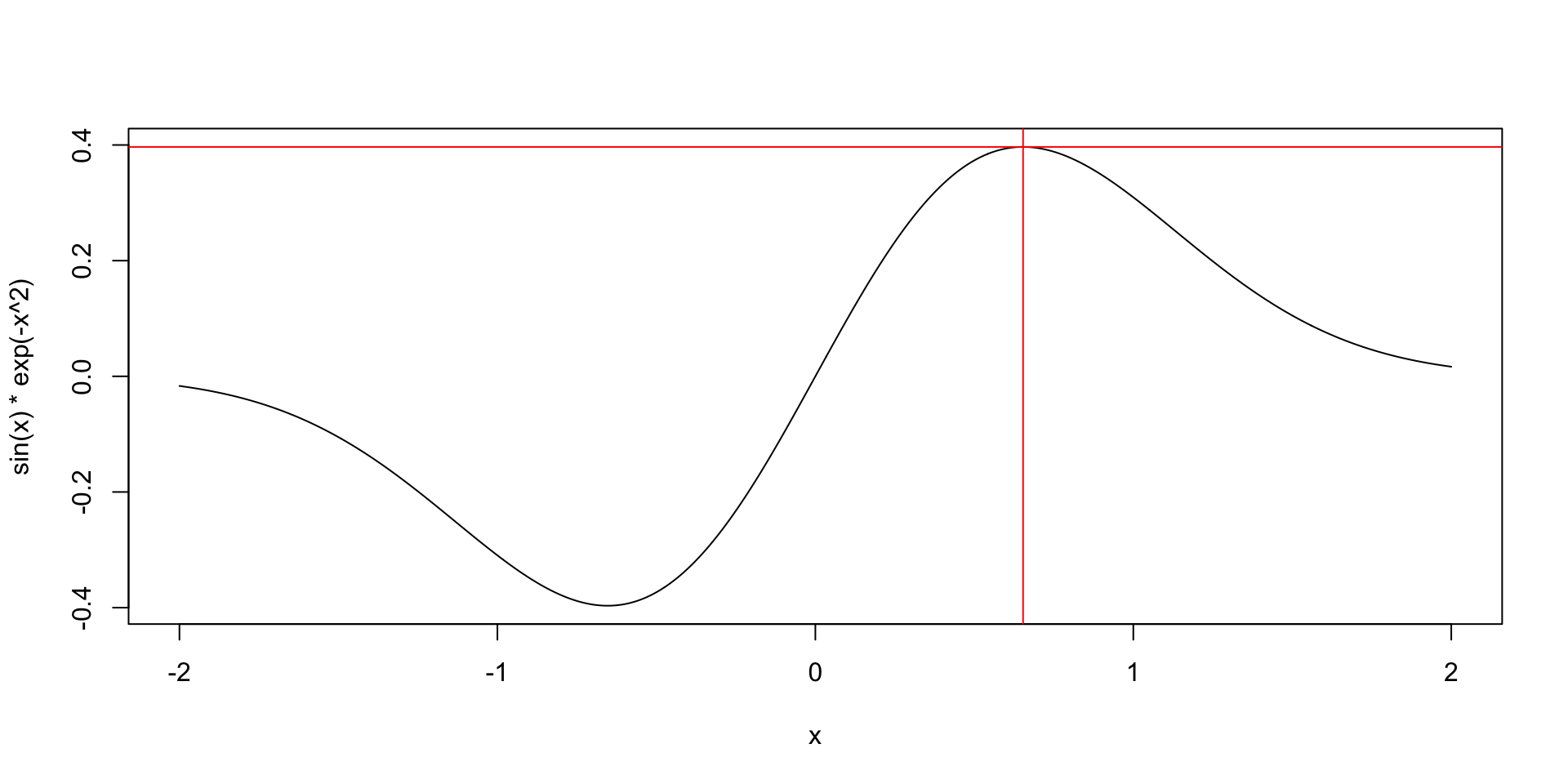
Simple example
- Find the maximum value of \(f(x) = \sin(x)e^{-x^2}\).
Spring motion
- This differential equation describes how a spring moves over time.
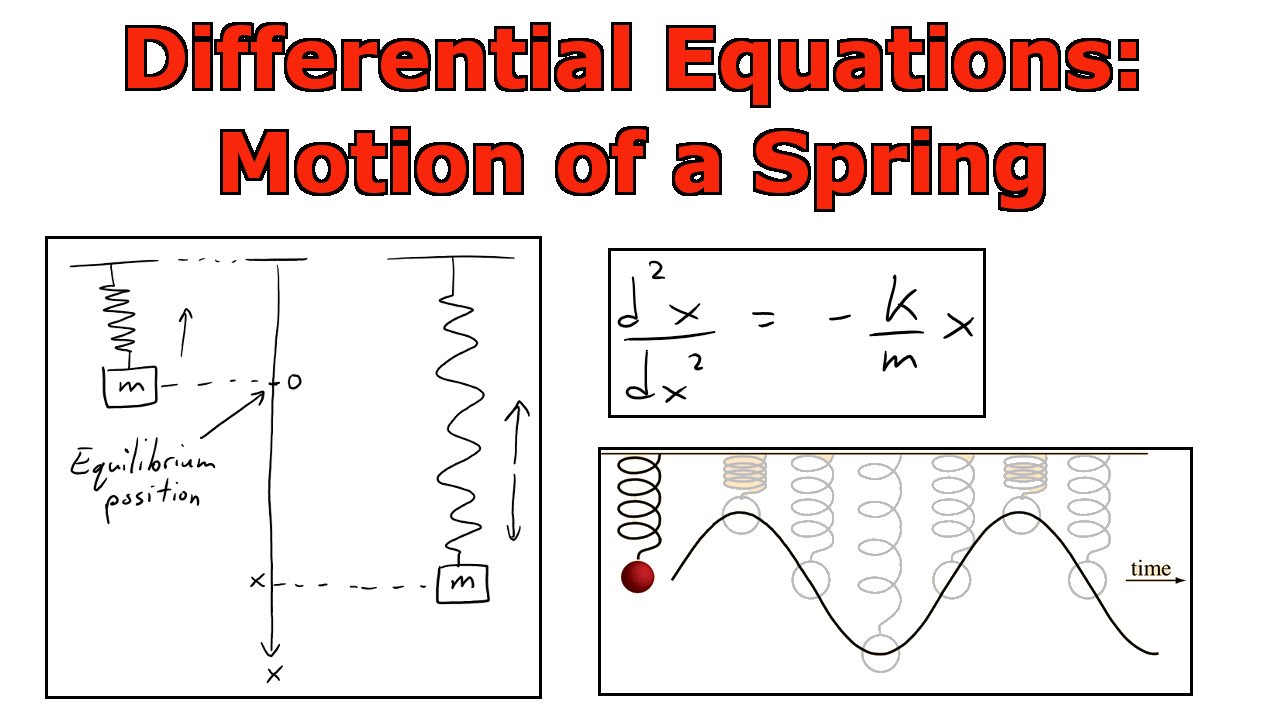
- Through math magic, we can figure out that the curve traced out by the spring position has to be \[ f(x) = A\cos(\omega t) + B \sin(\omega t) \]
- Where \(A\) and \(B\) are real numbers that are determined by where the spring starts and its initial speed.
- Since we know this, we can make a plot of the spring movement.
# Parameters
omega <- 4 * pi  # angular frequency = sqrt(k / m)
A <- -2          # initial displacement
B <- 1 / omega         # initial velocity divided by omega

# Time vector
t <- seq(0, 2, by = 0.01)  # 0 to 2 seconds

# Analytical solution
x <- A * cos(omega * t) + B * sin(omega * t)

# Plot
plot(t, x, type = "l", col = "blue", lwd = 2,
     xlab = "Time (seconds)", ylab = "Position",
     main = "Spring movement")
abline(h = 0, col = "gray", lty = 2)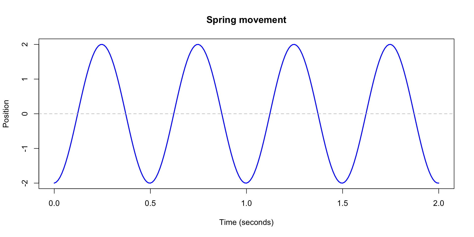
- So what do we do if we don’t know the math magic?
- We use a numerical solver. In R, the best one is in the
deSolvepackage. These are tools that use good approximations to get the solution. - The only downside is that we have to write our code in a very specific way.
# We have to do some transformations to make this DE work with deSolve
# but you can ignore that for now or you can google "transform a second order
# DE into system of first order DEs" if you want.
library(deSolve)

# Function for our DE (system)
spring_ode <- function(t, state, parameters) {
  with(as.list(c(state, parameters)), {
    dx1 <- x2
    dx2 <- -omega^2 * x1

    list(c(dx1, dx2))
  })
}

# Initial state: x(0) = -2, dx/dt(0) = 1
state <- c(x1 = -2, x2 = 1)

# Time points to solve for
times <- seq(0, 2, by = 0.01)

# Parameters list
parameters <- c(omega = omega)

# Solve ODE
out <- ode(y = state, times = times, func = spring_ode, parms = parameters)
str(out)
'deSolve' num [1:201, 1:3] 0 0.01 0.02 0.03 0.04 0.05 0.06 0.07 0.08 0.09 ...
- attr(*, "dimnames")=List of 2
..$ : NULL
..$ : chr [1:3] "time" "x1" "x2"
- attr(*, "istate")= int [1:21] 2 222 449 NA 6 6 0 52 22 NA ...
- attr(*, "rstate")= num [1:5] 0.01 0.01 2.01 0 0
- attr(*, "lengthvar")= int 2
- attr(*, "type")= chr "lsoda"- We can plot the solution to make sure it looks the same too.
# Convert to data frame
out_df <- as.data.frame(out)

# Plot displacement vs time
plot(out_df$time, out_df$x1, type = "l", col = "red", lwd = 3,
     xlab = "Time (seconds)", ylab = "Position",
     main = "Numerical Solution of spring movement")
lines(t, x, col = "blue", lty = 2, lwd = 2)

abline(h = 0, col = "gray", lty = 2)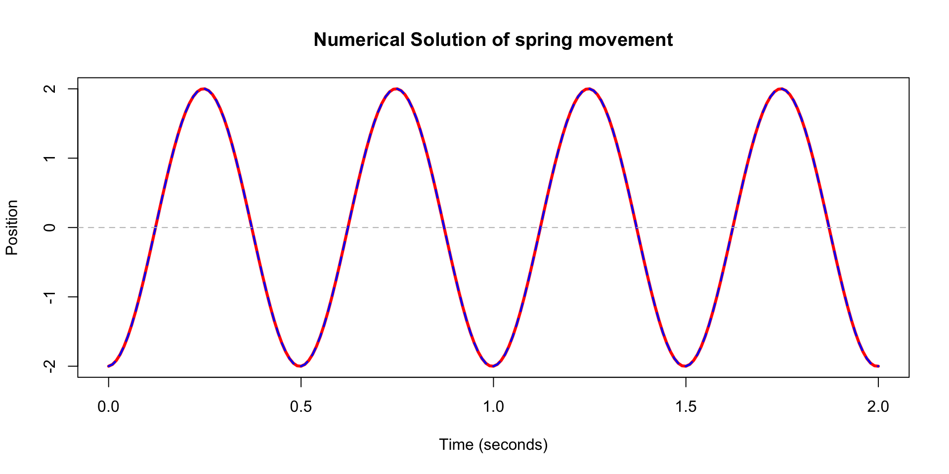
- They are exactly the same.
Compartment models
- If we divide up a population into states or compartments, usually we can write down how we expect people to move between those compartments.
- For example, consider the famous SIR model.
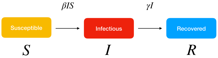
Source: DOI 10.3390/sym14122583
- You don’t need any math magic to write down differential equations from this model, you just need some training on how to read it.
\[ \begin{aligned} \frac{dS}{dt} &= -\beta I S \\ \frac{dI}{dt} &= \beta I S - \gamma I \\ \frac{dR}{dt} &= \gamma I \end{aligned} \]
- It is a true fact about differential equations that most (systems/equations) are impossible to solve via math magic, and we must resort to numerical solutions.
- It is impossible to solve the SIR system analytically with normal math magic, although it is possible using functions you’ve never heard of.
SIR model in deSolve
- Let’s walk through an example of solving SIR in deSolve.
- We need the following things to give to DSAIDE: a set of time points to evaluate our system at, a list of parameters of the system, an initial condition/state that describes the component populations at time \(0\), and a function that uses all of those things to update the system.
- Parameters: \(\beta\) (the force of infection) and \(\gamma\) (the recovery rate). I’ll arbitrarily set \(\beta = 0.01\) and \(\gamma = 0.5\) since I know it will make a good picture.
- Time points: it doesn’t really matter what we choose as long as it goes far enough out to see the patterns we’re interest in and is fine-grained enough to get good detail. For this problem we’ll use times of \(t = 0, 0.01, 0.02, \ldots, 9.99, 10\). Choosing the right ones usually takes some trial and error. Running more time points can take a really long time for complicated models.
- Initial state: we need how many susceptible, infected, and recovered people at time \(0\). Let’s say 1000 S, 1 I, and 0 R. Note you need at least one infected person to have an epidemic!
- A function. This is the tricky bit, and we have to write it kind of weird. We can leave out that weird
with()thing from before, but it does make your life easier so I recommend learning it.
sir_ode <- function(t, y, parameters) {
    # If you don't use with() you have to do this
    b <- parameters["beta"]
    g <- parameters["gamma"]

    S <- y["S"]
    I <- y["I"]
    R <- y["R"]

    dS <- -b * I * S
    dI <- b * I * S - g * I
    dR <- g * I

    # For deSolve the output always has to be a list like this
    out <- list(c(dS, dI, dR))
    return(out)
}- Now we should be able to call
deSolveand get a solution.
sir_soln <- deSolve::ode(
    y = sir_initial_condition,
    times = t_seq,
    func = sir_ode,
    parms = sir_parms
)
head(sir_soln)| time | S | I | R |
|---|---|---|---|
| 0.00 | 1000.0000 | 1.000000 | 0.0000000 |
| 0.01 | 999.8951 | 1.099654 | 0.0052452 |
| 0.02 | 999.7798 | 1.209224 | 0.0110131 |
| 0.03 | 999.6529 | 1.329698 | 0.0173557 |
| 0.04 | 999.5135 | 1.462153 | 0.0243301 |
| 0.05 | 999.3602 | 1.607779 | 0.0319991 |
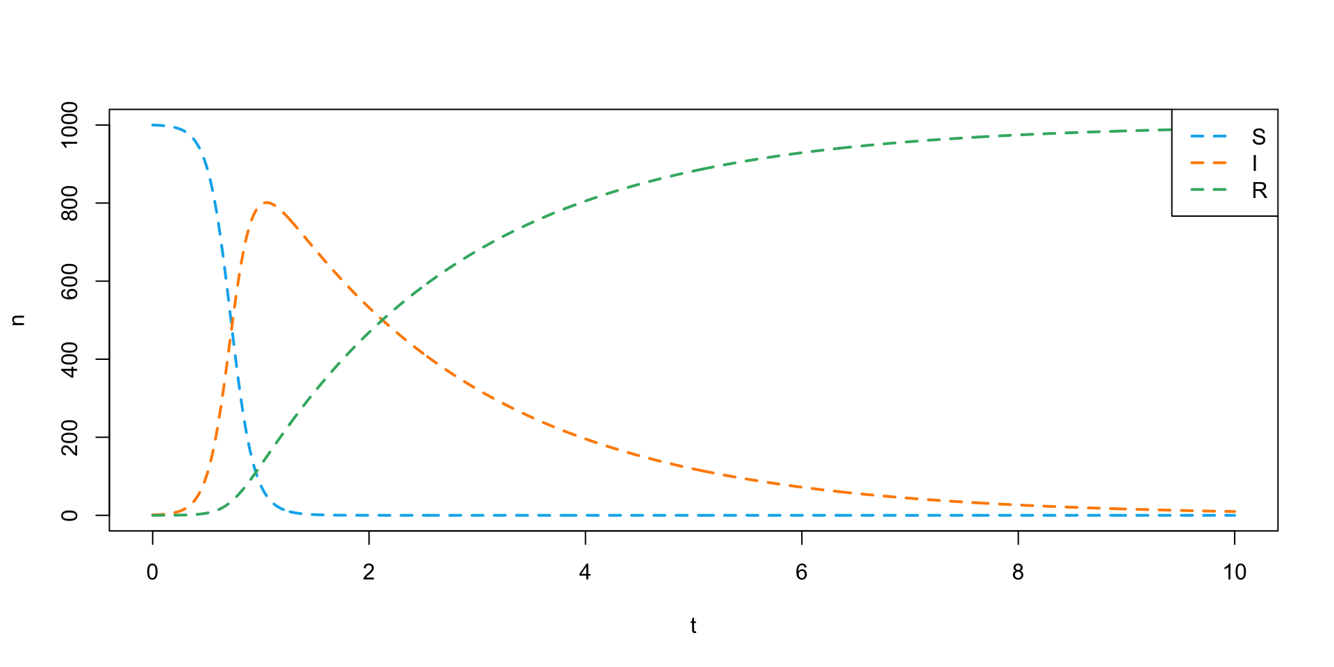
- Let’s plot the solution.
plot(
    NULL, NULL,
    xlim = c(0, 10), ylim = c(0, 1000),
    xlab = "t", ylab = "n"
)
my_colors <- c("deepskyblue2", "darkorange", "mediumseagreen")

lines(sir_soln[,"time"], sir_soln[,"S"], col = my_colors[1], lwd = 2, lty = 2)
lines(sir_soln[,"time"], sir_soln[,"I"], col = my_colors[2], lwd = 2, lty = 2)
lines(sir_soln[,"time"], sir_soln[,"R"], col = my_colors[3], lwd = 2, lty = 2)
legend(
    "topright",
    legend = c("S", "I", "R"),
    lty = 2, lwd = 2, col = my_colors
)
You try it!
- Update your model slightly so that people who are Recovered can become Susceptible again over time. This is called a SIRS model. It looks like this.
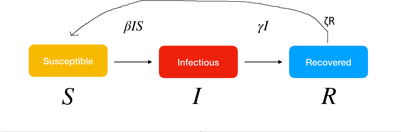
- Hint: the system of equations implied by my incredible drawing is:
\[ \begin{aligned} \frac{dS}{dt} &= -\beta I S + \zeta R\\ \frac{dI}{dt} &= \beta I S - \gamma I \\ \frac{dR}{dt} &= \gamma I - \zeta R \end{aligned} \]
- Hint: you need to add another parameter and update the function, but you don’t need to change anything about the initial state or time values (if you don’t want to).
- Solution!
sirs_initial_condition <- sir_initial_condition
sirs_t <- seq(0, 1000, 0.01)
sirs_parms <- c(sir_parms, zeta = 0.25)
sirs_ode <- function(t, y, parameters) {
    # If you don't use with() you have to do this
    b <- parameters["beta"]
    g <- parameters["gamma"]
    z <- parameters["zeta"]

    S <- y["S"]
    I <- y["I"]
    R <- y["R"]

    dS <- -b * I * S + z * R
    dI <- b * I * S - g * I
    dR <- g * I - z * R

    # For deSolve the output always has to be a list like this
    out <- list(c(dS, dI, dR))
    return(out)
}

sirs_soln <- deSolve::ode(
    y = sirs_initial_condition,
    times = sirs_t,
    func = sirs_ode,
    parms = sirs_parms
)
head(sirs_soln)| time | S | I | R |
|---|---|---|---|
| 0.00 | 1000.0000 | 1.000000 | 0.0000000 |
| 0.01 | 999.8951 | 1.099654 | 0.0052388 |
| 0.02 | 999.7798 | 1.209224 | 0.0109865 |
| 0.03 | 999.6530 | 1.329698 | 0.0172938 |
| 0.04 | 999.5136 | 1.462153 | 0.0242165 |
| 0.05 | 999.3604 | 1.607779 | 0.0318156 |
- Let’s plot this solution the same way.
plot(
    NULL, NULL,
    xlim = c(0, 10), ylim = c(0, 1000),
    xlab = "t", ylab = "n",
    main = "SIRS model solution"
)
my_colors <- c("deepskyblue2", "darkorange", "mediumseagreen")

lines(sirs_soln[,"time"], sirs_soln[,"S"], col = my_colors[1], lwd = 2, lty = 2)
lines(sirs_soln[,"time"], sirs_soln[,"I"], col = my_colors[2], lwd = 2, lty = 2)
lines(sirs_soln[,"time"], sirs_soln[,"R"], col = my_colors[3], lwd = 2, lty = 2)
legend(
    "topright",
    legend = c("S", "I", "R"),
    lty = 2, lwd = 2, col = my_colors
)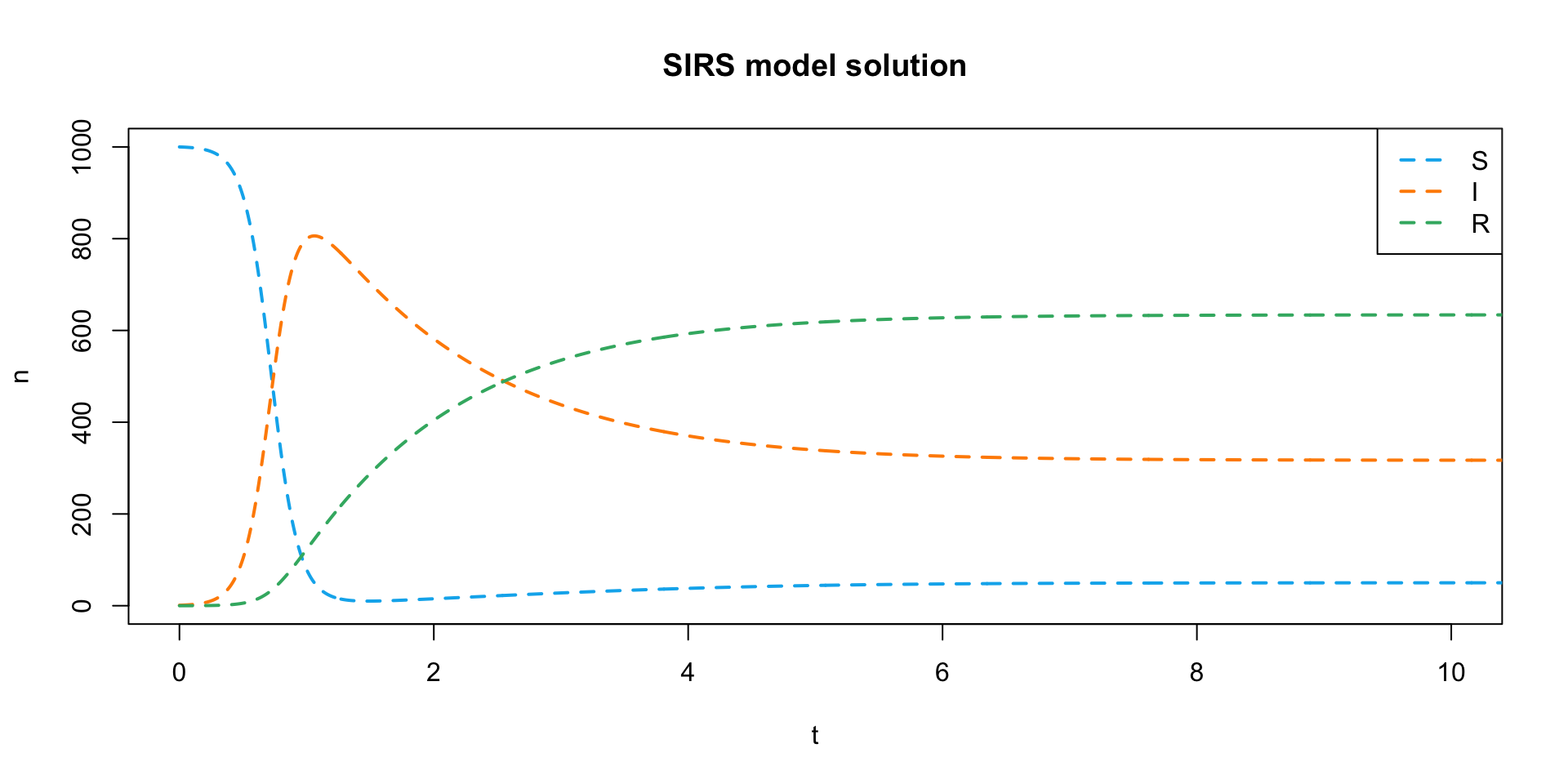
- By including the \(\zeta\) parameter, we get an endemic equilibrium instead of a disease-free equilibrium.
- This model can give you some other interesting oscillation patterns if you play with the parameters, but almost all parameter combinations will lead to a steady state.
You try it (problem 2)
- If you’re ready for another challenge, try solving the equations for this model where the pathogen is environmental.
- This model also includes a birth rate \(n\) (assuming all individuals are born into the susceptible compartment) and a death rate \(m\) that assumes people from the S, I, and R compartments all die at the same rate. If you want to, you can leave out any terms with \(m\) and \(n\) in them, they aren’t too important (or you can set them to 0 in your model).
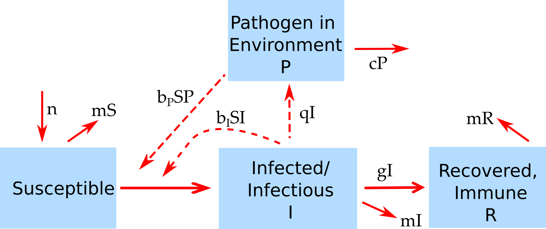 - Here are the equations implied by the model. \[
\begin{aligned}
\frac{dS}{dt} &= n - b_{I}IS - b_{P}PS -mS \\
\frac{dI}{dt} &= b_{I}IS + b_{I}PS -gI - mI\\
\frac{dR}{dt} &= gI - mR \\
\frac{dP}{dt} &= qI - cP
\end{aligned}
\]
- Here are the equations implied by the model. \[
\begin{aligned}
\frac{dS}{dt} &= n - b_{I}IS - b_{P}PS -mS \\
\frac{dI}{dt} &= b_{I}IS + b_{I}PS -gI - mI\\
\frac{dR}{dt} &= gI - mR \\
\frac{dP}{dt} &= qI - cP
\end{aligned}
\]
- No solution typed out for this problem. You can work on it on your own and email me questions, or if we have time we can work on it together.