Module XX: Bootstrapping can be easy and fun
Learning goals
- Understand the basics of bootstrapping – be able to construct your own bootstrap resamples and calculate a bootstrap CI for a statistic.
- Make your own bootstraps with loops or functional programming.
- Combine your own knowledge of R programming techniques with the
bootpackage for easy bootstrapping. - Use the
rsamplepackage and advanced R programming techniques to iterate over lists of bootstrap resamples.
What is bootstrapping?
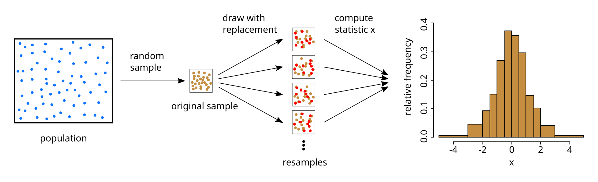
- bootstrapping is a method for obtaining standard error estimates or confidence intervals by resampling.
- We’ll specifically talk about the nonparametric bootstrap but there are entire books about bootstrap methods.
credit: https://commons.wikimedia.org/wiki/File:Illustration_bootstrap.svg
What is bootstrapping?
- We have some statistic \(\theta\) that we want to estimate from the dataset.
- We create \(B\) resamples of the dataset by randomly sampling from it, and then we calculate the statistic \(\theta_B\) on each dataset.
- If we create these resamples the correct way, the observed distribution of \(\theta_1, \ldots, \theta_B\) will converge to the true sampling distribution of \(\theta\).
- Specifically, we create a resample by sampling \(n\) (our sample size) rows from the original dataset with replacement.
What is bootstrapping?
- That’s math jargon to say that sometimes doing this resampling thing will give us better confidence intervals than normality assumptions.
- Usually bootstrapping works well for small datasets, estimates with complex (or nonexistant) standard error formulas, or for statistics with highly skewed distributions.
credit: https://commons.wikimedia.org/wiki/File:Illustration_bootstrap.svg
Low birthweight data and the data() function
- For this example, we’ll use a famous epidemiological dataset about babies with low birthweight.
- Many R packages have built-in datasets, which you can access with the
data()function. - The low birth weight dataset, called
birthwt, is in theMASSpackage, so you can access it with eitherMASS::birthwtordata("birthwt", package = "MASS").
Bootstrapping example
- Use bootstrapping to calculate a 95% CI for the risk difference in low birth weight (
low, 1 is low birth weight) between mothers who smoke (smoke = 1) and don’t (smoke= 0).
- First create the resamples. We need to use
set.seed()to make sure our results are the same every time we run our code!
set.seed(370)
B <- 1000
# Alternatively use replicate() if you don't like the weird function here
# or use a loop
resamples <- lapply(
    1:B,
    \(n) birthwt[sample.int(nrow(birthwt), replace = TRUE), ]
)

str(resamples, 1)
List of 1000
$ :'data.frame': 189 obs. of 10 variables:
$ :'data.frame': 189 obs. of 10 variables:
$ :'data.frame': 189 obs. of 10 variables:
$ :'data.frame': 189 obs. of 10 variables:
$ :'data.frame': 189 obs. of 10 variables:
$ :'data.frame': 189 obs. of 10 variables:
$ :'data.frame': 189 obs. of 10 variables:
$ :'data.frame': 189 obs. of 10 variables:
$ :'data.frame': 189 obs. of 10 variables:
$ :'data.frame': 189 obs. of 10 variables:
$ :'data.frame': 189 obs. of 10 variables:
$ :'data.frame': 189 obs. of 10 variables:
$ :'data.frame': 189 obs. of 10 variables:
$ :'data.frame': 189 obs. of 10 variables:
$ :'data.frame': 189 obs. of 10 variables:
$ :'data.frame': 189 obs. of 10 variables:
$ :'data.frame': 189 obs. of 10 variables:
$ :'data.frame': 189 obs. of 10 variables:
$ :'data.frame': 189 obs. of 10 variables:
$ :'data.frame': 189 obs. of 10 variables:
$ :'data.frame': 189 obs. of 10 variables:
$ :'data.frame': 189 obs. of 10 variables:
$ :'data.frame': 189 obs. of 10 variables:
$ :'data.frame': 189 obs. of 10 variables:
$ :'data.frame': 189 obs. of 10 variables:
$ :'data.frame': 189 obs. of 10 variables:
$ :'data.frame': 189 obs. of 10 variables:
$ :'data.frame': 189 obs. of 10 variables:
$ :'data.frame': 189 obs. of 10 variables:
$ :'data.frame': 189 obs. of 10 variables:
$ :'data.frame': 189 obs. of 10 variables:
$ :'data.frame': 189 obs. of 10 variables:
$ :'data.frame': 189 obs. of 10 variables:
$ :'data.frame': 189 obs. of 10 variables:
$ :'data.frame': 189 obs. of 10 variables:
$ :'data.frame': 189 obs. of 10 variables:
$ :'data.frame': 189 obs. of 10 variables:
$ :'data.frame': 189 obs. of 10 variables:
$ :'data.frame': 189 obs. of 10 variables:
$ :'data.frame': 189 obs. of 10 variables:
$ :'data.frame': 189 obs. of 10 variables:
$ :'data.frame': 189 obs. of 10 variables:
$ :'data.frame': 189 obs. of 10 variables:
$ :'data.frame': 189 obs. of 10 variables:
$ :'data.frame': 189 obs. of 10 variables:
$ :'data.frame': 189 obs. of 10 variables:
$ :'data.frame': 189 obs. of 10 variables:
$ :'data.frame': 189 obs. of 10 variables:
$ :'data.frame': 189 obs. of 10 variables:
$ :'data.frame': 189 obs. of 10 variables:
$ :'data.frame': 189 obs. of 10 variables:
$ :'data.frame': 189 obs. of 10 variables:
$ :'data.frame': 189 obs. of 10 variables:
$ :'data.frame': 189 obs. of 10 variables:
$ :'data.frame': 189 obs. of 10 variables:
$ :'data.frame': 189 obs. of 10 variables:
$ :'data.frame': 189 obs. of 10 variables:
$ :'data.frame': 189 obs. of 10 variables:
$ :'data.frame': 189 obs. of 10 variables:
$ :'data.frame': 189 obs. of 10 variables:
$ :'data.frame': 189 obs. of 10 variables:
$ :'data.frame': 189 obs. of 10 variables:
$ :'data.frame': 189 obs. of 10 variables:
$ :'data.frame': 189 obs. of 10 variables:
$ :'data.frame': 189 obs. of 10 variables:
$ :'data.frame': 189 obs. of 10 variables:
$ :'data.frame': 189 obs. of 10 variables:
$ :'data.frame': 189 obs. of 10 variables:
$ :'data.frame': 189 obs. of 10 variables:
$ :'data.frame': 189 obs. of 10 variables:
$ :'data.frame': 189 obs. of 10 variables:
$ :'data.frame': 189 obs. of 10 variables:
$ :'data.frame': 189 obs. of 10 variables:
$ :'data.frame': 189 obs. of 10 variables:
$ :'data.frame': 189 obs. of 10 variables:
$ :'data.frame': 189 obs. of 10 variables:
$ :'data.frame': 189 obs. of 10 variables:
$ :'data.frame': 189 obs. of 10 variables:
$ :'data.frame': 189 obs. of 10 variables:
$ :'data.frame': 189 obs. of 10 variables:
$ :'data.frame': 189 obs. of 10 variables:
$ :'data.frame': 189 obs. of 10 variables:
$ :'data.frame': 189 obs. of 10 variables:
$ :'data.frame': 189 obs. of 10 variables:
$ :'data.frame': 189 obs. of 10 variables:
$ :'data.frame': 189 obs. of 10 variables:
$ :'data.frame': 189 obs. of 10 variables:
$ :'data.frame': 189 obs. of 10 variables:
$ :'data.frame': 189 obs. of 10 variables:
$ :'data.frame': 189 obs. of 10 variables:
$ :'data.frame': 189 obs. of 10 variables:
$ :'data.frame': 189 obs. of 10 variables:
$ :'data.frame': 189 obs. of 10 variables:
$ :'data.frame': 189 obs. of 10 variables:
$ :'data.frame': 189 obs. of 10 variables:
$ :'data.frame': 189 obs. of 10 variables:
$ :'data.frame': 189 obs. of 10 variables:
$ :'data.frame': 189 obs. of 10 variables:
$ :'data.frame': 189 obs. of 10 variables:
[list output truncated]- Now write a function to calculate the statistic.
- Make sure to calculate the point estimate on the entire dataset as well.
- Now calculate the statistic on every resample.
- Now we have to calculate the SE. There are a few different ways. First is the normal method, where we calculate the standard error from the bootstrap distribution.
- This is just the standard deviation of the bootstrap estimates. Then we calculate the normal-approximate CI as usual.
- That method is kind of bad, but common. A better method is the percentile method which uses the quantiles of the bootstrap estimates.
- In this case they’re the same because this RD is easy to estimate. But that won’t always be true!
You try it!
- Look up the formula for the standard error of the risk ratio.
- Calculate the risk ratio for low birthweight in mothers with (
ht= 1) and without (ht = 0) a history of hypertension using the standard CI, and using a bootstrap CI with the percentile method.
- Hint:
- Hint: the formula for the SE of the log risk ratio is \[ \sqrt{\bigg( \frac{1}{a} + \frac{1}{c} \bigg) - \bigg( \frac{1}{a+b} + \frac{1}{c+d} \bigg)} \]
for a \(2\times2\) table.
| Exposed | Unexposed | |
|---|---|---|
| Exposed | a | b |
| Unexposed | c | d |
- Solution: first we calculate the point estimate and the Wald-type CI based on the SE formula.
point_estimate_rr <- rr_ht(birthwt)
contigency_table_ht <- table(
    factor(birthwt$ht, c(1, 0), c("Exposed", "Unexposed")),
    factor(birthwt$smoke, c(1, 0), c("Case", "Control"))
)

calculate_log_rr_se <- function(contigency_table) {
    a <- contigency_table[1, 1]
    b <- contigency_table[1, 2]
    c <- contigency_table[2, 1]
    d <- contigency_table[2, 2]

    se <- sqrt((1/a + 1/c) - (1/(a+b) + 1/(c+d)))
    return(se)
}
log_rr_se <- calculate_log_rr_se(contigency_table_ht)
# It's on the log scale, so we have to calculate the CI like this!
exp(log_rr_se * c(-1.96, 1.96) + log(point_estimate_rr))
[1] 0.9915692 3.9760368- Solution: now we do the bootstrap CI.
Bootstrapping multiple statistics at one time
- If our bootstrap function returns a
vector, we can get multiple statistics at once.
get_smoking_stats <- function(resample) {
    risk_smoke <- mean(resample$low[resample$smoke == 1])
    risk_no_smoke <- mean(resample$low[resample$smoke == 0])

    odds_smoke <- risk_smoke / (1 - risk_smoke)
    odds_no_smoke <- risk_no_smoke / (1 - risk_no_smoke)

    rd <- risk_smoke - risk_no_smoke
    rr <- risk_smoke / risk_no_smoke
    or <- odds_smoke / odds_no_smoke

    out <- c(
        "Risk difference" = rd,
        "Risk ratio" = rr,
        "Odds ratio" = or
    )
    return(out)
}

smoking_stats <- sapply(resamples, get_smoking_stats)
str(smoking_stats)
num [1:3, 1:1000] 0.2051 2.0082 2.7044 0.0224 1.0879 ...
- attr(*, "dimnames")=List of 2
..$ : chr [1:3] "Risk difference" "Risk ratio" "Odds ratio"
..$ : NULL- The output looks really confusing. But it’s a matrix so we can use
apply()!
point_estimates <- get_smoking_stats(birthwt)
boot_cis <- apply(smoking_stats, 1, \(x) quantile(x, c(0.025, 0.975)))

# Just some code to show everything neatly
rbind(
    "Lower" = boot_cis[1, ],
    "Point" = point_estimates,
    "Upper" = boot_cis[2, ]
) |>
    t() |>
round(digits = 2)| Lower | Point | Upper | |
|---|---|---|---|
| Risk difference | 0.01 | 0.15 | 0.30 |
| Risk ratio | 1.04 | 1.61 | 2.57 |
| Odds ratio | 1.05 | 2.02 | 4.18 |
Errors in bootstrapping and the boot package
- The situations we just observed are pretty simple, and our bootstrap estimates are pretty trustworthy (they would be more trustworthy if we increased
B, a good rule of thumb is 1,000 just for you, 10,000 for your boss, and 100,000 for a paper if it’s feasible). - But in some situations, bootstrapping can be biased. There is a fix for this called the “BCa” bootstrap.
- BCa is hard to do by hand, but easy to do with the
bootpackage.
The boot package
- We have to write our function a certain way for
boot. It must have two arguments, the first is the data, and the second is a list of indices that are included in a resample.
boot_smoking_stats <- function(data, idx) {
    resample <- data[idx, ]
    out <- get_smoking_stats(resample)
    return(out)
}

library(boot)
bootstraps_smoking <- boot::boot(birthwt, boot_smoking_stats, R = 1000)
bootstraps_smoking
ORDINARY NONPARAMETRIC BOOTSTRAP


Call:
boot::boot(data = birthwt, statistic = boot_smoking_stats, R = 1000)


Bootstrap Statistics :
     original       bias    std. error
t1* 0.1532315 0.0009951909  0.07034402
t2* 1.6076421 0.0444346127  0.35834007
t3* 2.0219436 0.1290172225 0.71556649- We can see this calculates the point estimate, bias, and boostrap SE for us. The bias is what we didn’t know how to calculate before.
- We can easily compare multiple CI methods with
boot. - For technical reasons that are too complicated to talk about, when you do multiple stats at one time in
boot, you must always manually set theindexargument.
Warning in boot::boot.ci(bootstraps_smoking, index = 1): bootstrap variances
needed for studentized intervals
BOOTSTRAP CONFIDENCE INTERVAL CALCULATIONS
Based on 1000 bootstrap replicates
CALL :
boot::boot.ci(boot.out = bootstraps_smoking, index = 1)
Intervals :
Level Normal Basic
95% ( 0.0144, 0.2901 ) ( 0.0200, 0.2876 )
Level Percentile BCa
95% ( 0.0189, 0.2864 ) ( 0.0153, 0.2834 )
Calculations and Intervals on Original Scale- Of course, we can use loops or FP to do this for all of our statistics.
smoking_point_estimates <- bootstraps_smoking$t0
smoking_cis_list <- lapply(
    1:length(smoking_point_estimates),
    \(i) boot::boot.ci(bootstraps_smoking, type = "bca", index = i)
)
str(smoking_cis_list, 1)
List of 3
$ :List of 4
..- attr(*, "class")= chr "bootci"
$ :List of 4
..- attr(*, "class")= chr "bootci"
$ :List of 4
..- attr(*, "class")= chr "bootci"- Cleaning them up is kind of difficult, this is a weirdly formatted S3 object.
smoking_cis <- sapply(
    smoking_cis_list,
    \(x) x$bca[4:5]
)

# Same cleanup code as before
rbind(
    "lower" = smoking_cis[1, ],
    "point" = smoking_point_estimates,
    "upper" = smoking_cis[2, ]
) |>
    t() |>
round(digits = 2)| lower | point | upper | |
|---|---|---|---|
| Risk difference | 0.02 | 0.15 | 0.28 |
| Risk ratio | 1.05 | 1.61 | 2.42 |
| Odds ratio | 1.07 | 2.02 | 3.67 |
You try it!
- Fit a logistic regression model to predict low birth weight using this dataset. Use any predictors in the dataset that you think are relevant.
- Get the standard confidence intervals using the profile method (that is, with
confint()). - Get bootstrap estimates for the coefficients.
- Do the bootstrap estimates lead you to the same interpretation, or a different interpretation?
(No solution typed up for this problem, if we have time/interest we can cover it together.)