Module XX: Power 2 (Unlimited Power)
Calculating power
- For this example, we’ll use birthweight data from the
MASSpackage, calledbirthwt. You can load this data using thedata()function.
- Let’s do a two sample \(t\)-test for birth weight (
bwt) for mothers who smoke and don’t smoke (smoke).
    Welch Two Sample t-test

data:  bwt by smoke
t = 2.7299, df = 170.1, p-value = 0.007003
alternative hypothesis: true difference in means between group 0 and group 1 is not equal to 0
95 percent confidence interval:
  78.57486 488.97860
sample estimates:
mean in group 0 mean in group 1
3055.696 2771.919 - We can also calculate the power of this test. It takes a little bit of finagling, but it’s not too hard.
- You could also use G Power to do this, and it would probably be easier.
- Side note: aggregate is a great way to use formulas for grouped calculations.
group_sample_sizes <- aggregate(bwt ~ smoke, data = birthwt, FUN = length)
group_means <- aggregate(bwt ~ smoke, data = birthwt, FUN = mean)
group_sds <- aggregate(bwt ~ smoke, data = birthwt, FUN = sd)
power.t.test(
    # Use the average group sample size
    n = mean(group_sample_sizes$bwt),
    # d = TRUE difference in means / so we use our post-hoc observation
    delta = diff(group_means$bwt),
    # Pool the SD's
    sd = sqrt(mean(group_sds$bwt ^ 2)),
    # Alpha level of test
    sig.level = 0.05,
    # Details about the test
    type = "two.sample",
    alternative = "two.sided"
)
     Two-sample t test power calculation

              n = 94.5
          delta = 283.7767
             sd = 707.6758
      sig.level = 0.05
          power = 0.7829694
    alternative = two.sided

NOTE: n is number in *each* group- We can an estimated power of about 78%. Of course this is post-hoc power so it’s basically useless.
- The G Power calculation is actually a bit more flexible.
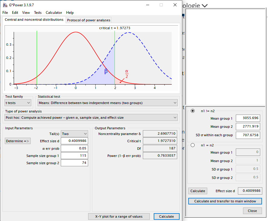
- The estimate is a bit different because of how G Power deals with unequal sample sizes between groups.
Power curves
- We can often get a good idea about the SD from the literature or from knowledge about how our assay/measurement works, so we’ll ignore that for now (it is harder for observational studies than for experiments).
- But in general we have no idea what the effect size (difference in means) should be before we do the study. So how do we get the power or sample size?
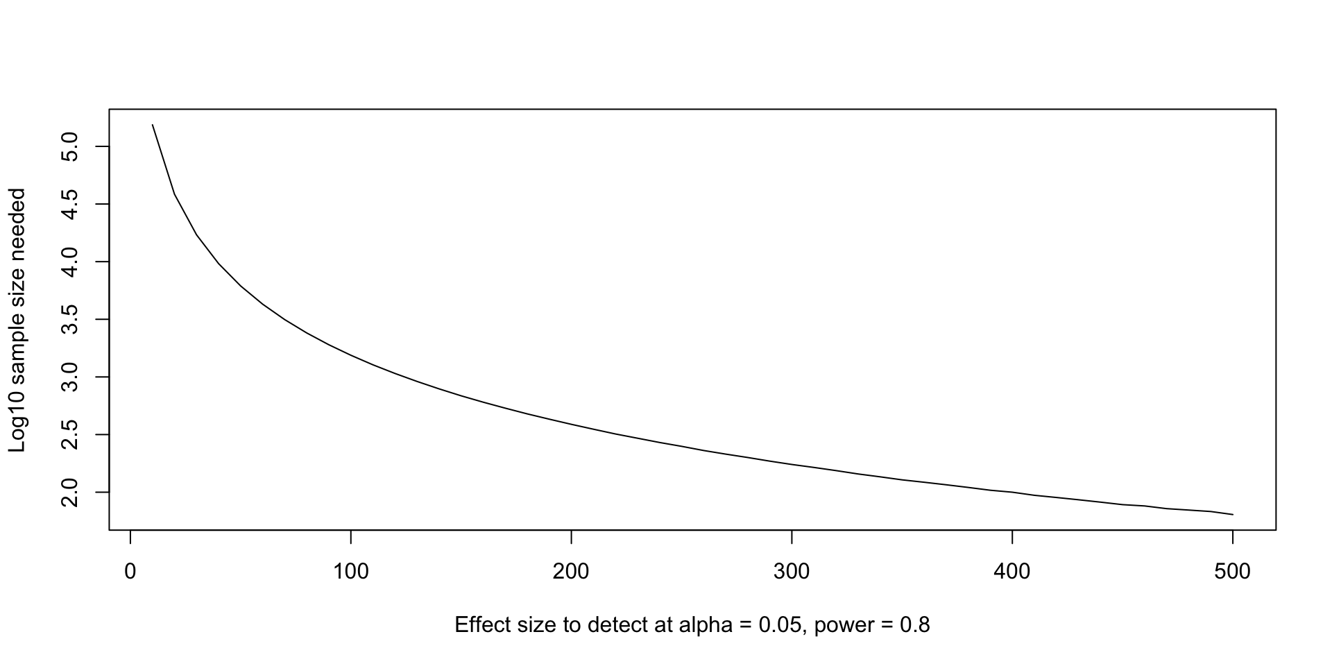
- We can calculate the required sample size to achieve multiple different effect sizes. For the
birthwtexample, let’s pretend we didn’t run our study yet, but we know that the pooled sd should be around 700. Let’s calculate the sample size needed to achieve 80% power at multiple effect sizes. - In real life, maybe we can get this magical 700 number from previous studies or preliminary data.
- We can use the tools we’ve learned to get many different sample size calculations.
effect_sizes <- seq(10, 500, 10)
sample_size_calc <- lapply(
    effect_sizes,
    \(d) power.t.test(delta = d, sd = 700, sig.level = 0.05, power = 0.80)
)
str(sample_size_calc, 1)
List of 50
$ :List of 8
..- attr(*, "class")= chr "power.htest"
$ :List of 8
..- attr(*, "class")= chr "power.htest"
$ :List of 8
..- attr(*, "class")= chr "power.htest"
$ :List of 8
..- attr(*, "class")= chr "power.htest"
$ :List of 8
..- attr(*, "class")= chr "power.htest"
$ :List of 8
..- attr(*, "class")= chr "power.htest"
$ :List of 8
..- attr(*, "class")= chr "power.htest"
$ :List of 8
..- attr(*, "class")= chr "power.htest"
$ :List of 8
..- attr(*, "class")= chr "power.htest"
$ :List of 8
..- attr(*, "class")= chr "power.htest"
$ :List of 8
..- attr(*, "class")= chr "power.htest"
$ :List of 8
..- attr(*, "class")= chr "power.htest"
$ :List of 8
..- attr(*, "class")= chr "power.htest"
$ :List of 8
..- attr(*, "class")= chr "power.htest"
$ :List of 8
..- attr(*, "class")= chr "power.htest"
$ :List of 8
..- attr(*, "class")= chr "power.htest"
$ :List of 8
..- attr(*, "class")= chr "power.htest"
$ :List of 8
..- attr(*, "class")= chr "power.htest"
$ :List of 8
..- attr(*, "class")= chr "power.htest"
$ :List of 8
..- attr(*, "class")= chr "power.htest"
$ :List of 8
..- attr(*, "class")= chr "power.htest"
$ :List of 8
..- attr(*, "class")= chr "power.htest"
$ :List of 8
..- attr(*, "class")= chr "power.htest"
$ :List of 8
..- attr(*, "class")= chr "power.htest"
$ :List of 8
..- attr(*, "class")= chr "power.htest"
$ :List of 8
..- attr(*, "class")= chr "power.htest"
$ :List of 8
..- attr(*, "class")= chr "power.htest"
$ :List of 8
..- attr(*, "class")= chr "power.htest"
$ :List of 8
..- attr(*, "class")= chr "power.htest"
$ :List of 8
..- attr(*, "class")= chr "power.htest"
$ :List of 8
..- attr(*, "class")= chr "power.htest"
$ :List of 8
..- attr(*, "class")= chr "power.htest"
$ :List of 8
..- attr(*, "class")= chr "power.htest"
$ :List of 8
..- attr(*, "class")= chr "power.htest"
$ :List of 8
..- attr(*, "class")= chr "power.htest"
$ :List of 8
..- attr(*, "class")= chr "power.htest"
$ :List of 8
..- attr(*, "class")= chr "power.htest"
$ :List of 8
..- attr(*, "class")= chr "power.htest"
$ :List of 8
..- attr(*, "class")= chr "power.htest"
$ :List of 8
..- attr(*, "class")= chr "power.htest"
$ :List of 8
..- attr(*, "class")= chr "power.htest"
$ :List of 8
..- attr(*, "class")= chr "power.htest"
$ :List of 8
..- attr(*, "class")= chr "power.htest"
$ :List of 8
..- attr(*, "class")= chr "power.htest"
$ :List of 8
..- attr(*, "class")= chr "power.htest"
$ :List of 8
..- attr(*, "class")= chr "power.htest"
$ :List of 8
..- attr(*, "class")= chr "power.htest"
$ :List of 8
..- attr(*, "class")= chr "power.htest"
$ :List of 8
..- attr(*, "class")= chr "power.htest"
$ :List of 8
..- attr(*, "class")= chr "power.htest"- But how do we get the sample size out of each power object thing? Fortunately
power.t.test()returns an S3 object of classpower.htest, and the documentation tells us how to get the quantities we want. - We also want to round the estimate up to the nearest whole number and (optionally, but I prefer this) multiply by two for the total sample size.
You try it! Power contours
- If we’re willing to do a little bit more wrangling, we can also do this for multiple variances.
- Here’s some code to help you get started, and then you can try to calculate the sample sizes yourself. First, make a grid of all the effect size and variance combinations we want to try.
- Note that the more values of delta and SD you want to try, the grid can become huge really quickly which could take a long time to run.
- Now because they are in a grid, you can do a 1-dimensional loop or
lapply(), instead of having to do a nested one, just iterate over the number of rows in the grid.
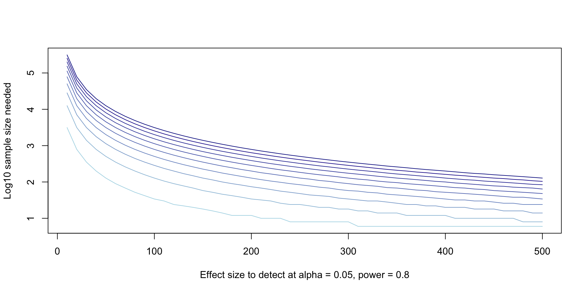
- My solution:
- There are two main ways people will try to plot these curves. One is by plotting a different colored curve for each SD.
plot(
    NULL, NULL,
    xlim = range(effect_sizes),
    ylim = range(log10(power_variables$sample_size)),
    xlab = "Effect size to detect at alpha = 0.05, power = 0.8",
    ylab = "Log10 sample size needed",
    type = "l"
)

variance_levels <- unique(power_variables$sd)
colors <- colorRampPalette(c("lightblue", "darkblue"))(length(variance_levels))
for (i in 1:length(variance_levels)) {
    sub <- subset(power_variables, sd == variance_levels[[i]])
    lines(x = sub$delta, y = log10(sub$sample_size), col = colors[[i]])
}
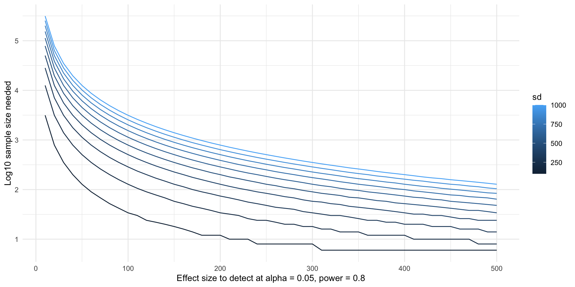
- If you know
ggplot2, this is way easier inggplot2.
- Mathematicians love to plot this as a “contour plot”. These are basically impossible to read but look impressive.
- This is insanely annoying to do in base R, so I’ll only show it in
ggplot2.
ggplot(power_variables) +
    aes(x = delta, y = sd, z = log10(sample_size)) +
    geom_contour_filled() +
    coord_cartesian(expand = FALSE) +
    labs(
        x = "Effect size to detect at alpha = 0.05, power = 0.8",
        y = "Assumed pooled SD",
        fill = "Log10 sample sized need"
    ) +
    theme_minimal() +
    theme(legend.position = "bottom")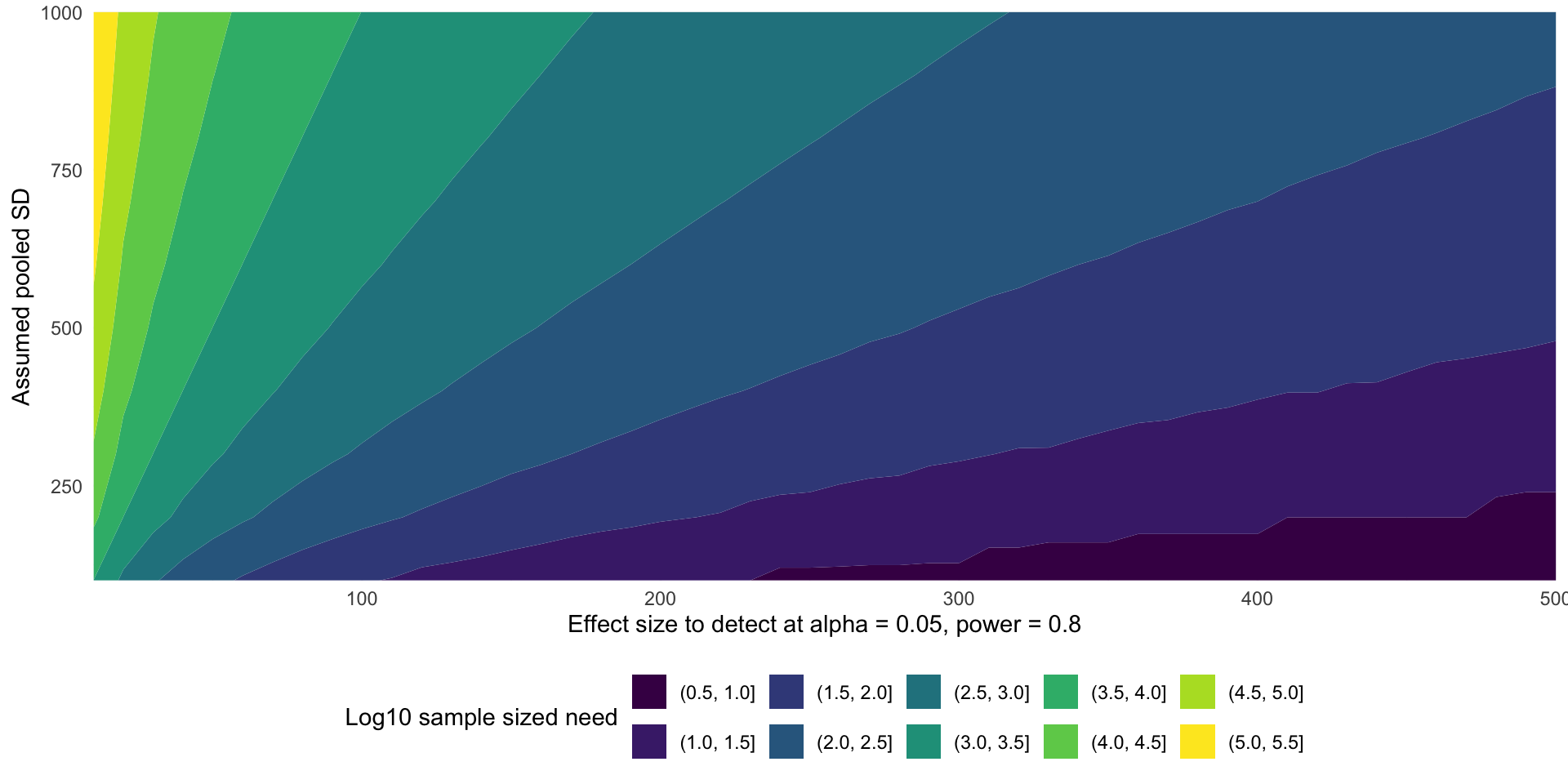
You try it!
- More often, we want to know what sample size it takes to get 80% power for a fixed leve
- The only way to do this by simulation is to try many sample sizes and do a simulation for each one.
- For the t-test example (this time you can assume the sample size for the two groups is the same to make life easier), make a plot of power vs. sample size, using the same group means and group SDs.
- Hint: write a function that simulates the data, does the t-tests, and gets which tests are rejections. Then,
lapply()this function over multiple values ofn(this is easy if you assumen1andn2are equal).
- Hint: here’s an outline for my function, and the code for how I used it.
- I returned the entire vector of TRUE/FALSE for rejections from the function, because I thought this was a convenient way to handle the data. You can do the sum() or mean() inside of the function and return a single number if you prefer that.
simulate_t_test_power <- function(N_sim, n1, n2, mu1, mu2, sd1, sd2, alpha = 0.05) {
simulated_data <-
replicate(
N_sims,
simulate_one_dataset(n1, n2, mu1, mu2, sd1, sd2),
simplify = FALSE
)
simulated_t_tests <- lapply(
simulated_data,
\(d) ...
)
simulation_p_values <- sapply(simulated_t_tests, ...)
rejected_h0 <- ...
return(rejected_h0)
}
n_per_group <- seq(...)
t_test_n_simulations <- sapply(
n_per_group,
\(n) simulate_t_test_power(
1000,
n, n,
mu1, mu2, sd1, sd2
)
)- Hint: after I ran this function, here’s how I got the power for each sample size.
- Here’s my solution.
simulate_t_test_power <- function(N_sim, n1, n2, mu1, mu2, sd1, sd2, alpha = 0.05) {
simulated_data <-
replicate(
N_sims,
simulate_one_dataset(n1, n2, mu1, mu2, sd1, sd2),
simplify = FALSE
)
simulated_t_tests <- lapply(
    simulated_data,
    \(d) t.test(d$group1, d$group2, conf.level = alpha)
)
simulation_p_values <- sapply(simulated_t_tests, \(x) x$p.value)
rejected_h0 <- simulation_p_values <= alpha
return(rejected_h0)
}
# You can do less of these
# and make N_sim lower
# if this takes too long
n_per_group <- seq(25, 250, 25)
set.seed(102)
t_test_n_simulations <- sapply(
n_per_group,
\(n) simulate_t_test_power(
1000,
n, n,
mu1, mu2, sd1, sd2
)
)
# sapply() gives us a matrix that we can easily apply() on to get summaries
# or use colMeans() cause its super fast and easy
res <- colMeans(t_test_n_simulations)
res [1] 0.3197 0.5670 0.7407 0.8495 0.9164 0.9576 0.9769 0.9880 0.9942 0.9976- By looking at these results, it’s clear where we can do a second simulation to hone in on a better sample size – between the 3rd and 4th levement of
n_per_groupwe get to our target.
# Interpolate between those two numbers, but don't repeat them
# cause we already did those sims!
n_per_group2 <- seq(n_per_group[3], n_per_group[4], 1)
n_per_group2_trim <- n_per_group2[2:(length(n_per_group2) - 1)]

set.seed(103)
t_test_n_simulations2 <- sapply(
    n_per_group2_trim,
    \(n) simulate_t_test_power(
        1000,
        n, n,
        mu1, mu2, sd1, sd2
    )
)

# sapply() gives us a matrix that we can easily apply() on to get summaries
# or use colMeans() cause its super fast and easy
res2 <- colMeans(t_test_n_simulations2)
res2
[1] 0.7448 0.7449 0.7681 0.7615 0.7647 0.7690 0.7764 0.7819 0.7814 0.7889
[11] 0.7952 0.8072 0.8007 0.8061 0.8180 0.8135 0.8149 0.8316 0.8313 0.8361
[21] 0.8410 0.8420 0.8463 0.8508- Now I’ll show you a neat trick to combine these simulations together and make a plot.
all_n <- c(n_per_group, n_per_group2_trim)
all_res <- c(res, res2)
sort_order <- order(all_n)

plot(
    all_n[sort_order], all_res[sort_order],
    type = "l",
    xlab = "Sample size", ylab = "Power"
)
# Find the smallest sample size with a power above 0.8
best_samp_size <- min(all_n[all_res > 0.8])
bss_power <- all_res[all_n == best_samp_size]

abline(h = bss_power, col = "red", lty = 2)
abline(v = best_samp_size, col = "red", lty = 2)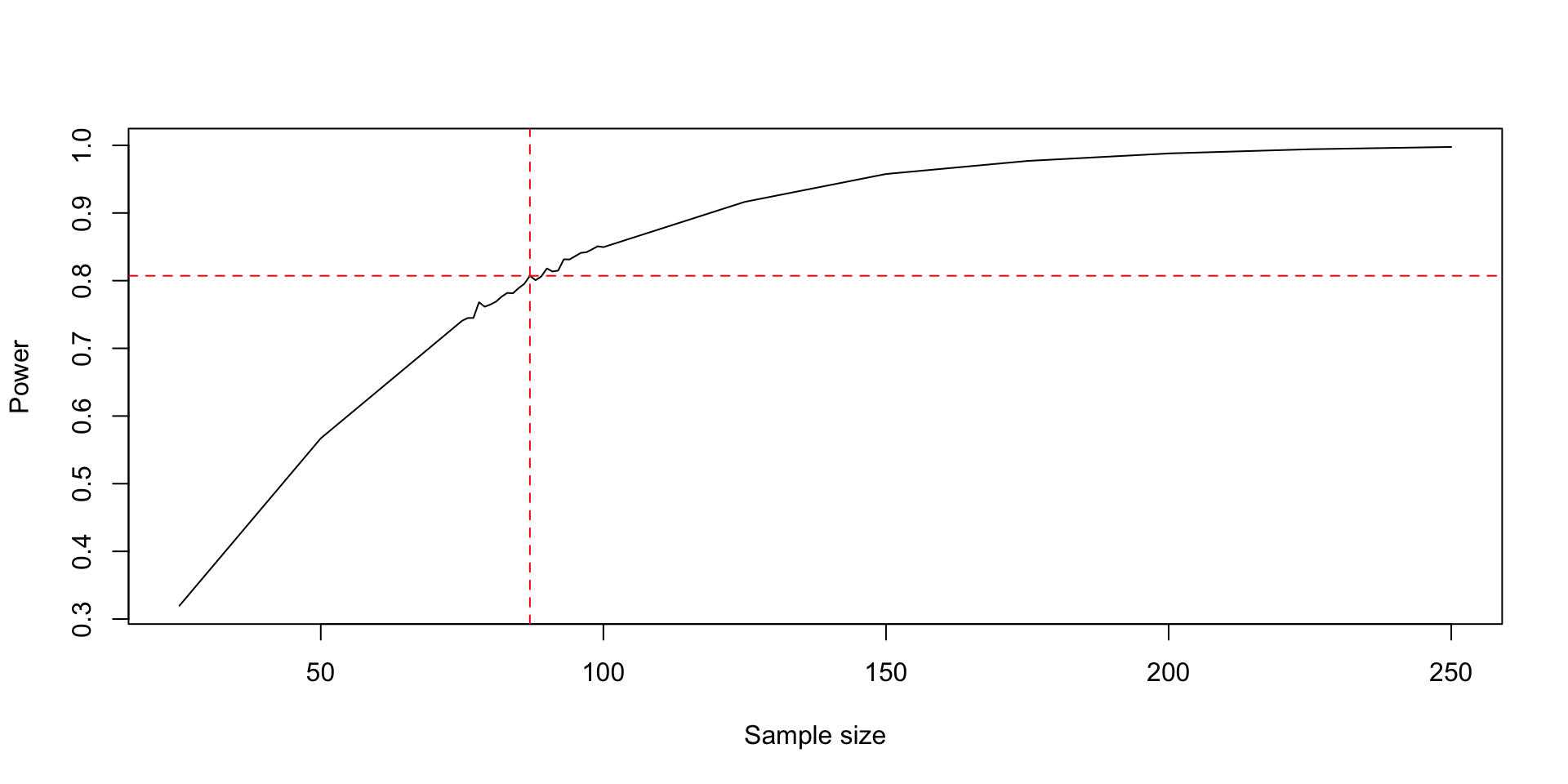
You try it! Finish the power simulation
- Now that we’ve walked through the building blocks, finish the power simulation. Find an \(n\) where the power under our assumptions about the data is between \(0.75\) and \(0.85\), that range is close enough.
- Hint: this kind of power simulation is easier if you break it down into components, write a function for each component, and then put them all together.
- I think you need three components: a data simulation function that returns a data set, a test function that returns a p-value for the given dataset (or returns accept/reject), and a function that puts those two parts together so you can repeat the whole thing.
- Hint: here’s the test function.
- Hint: now you can put the two parts together and then get the rejections.
- Hint: here’s my completed function.
- Can you repeat it for multiple
nvalues now?
logistic_power_simulation <- function(
        N_sims, n, beta_0, beta_1, exposure_prevalence, alpha
) {
    simulated_datasets <- replicate(
        N_sims,
        generate_logistic_model_data(n, beta_0, beta_1, exposure_prevalence),
        simplify = FALSE
    )

    simulated_p_values <- sapply(
        simulated_datasets,
        get_exposure_slope_p_value
    )

    rejections <- simulated_p_values <= alpha

    return(rejections)
}
n_values <- seq(25, 250, 25)
set.seed(110)
logistic_sim <- sapply(
n_values,
\(n) logistic_power_simulation(
1000,
n,
-2.2, 1.5, 0.4, 0.05
)
)
logistic_sim_power <- colMeans(logistic_sim)
plot(
n_values, logistic_sim_power,
xlab = "Sample size", ylab = "Power",
type = "l"
)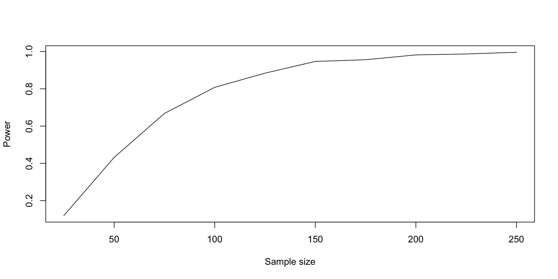
- If we look at the values, we see that a sample size of 100 gives us a power of about \(81\%\) under these assumptions.