Power and Sample Size

Lets import our package for these calculations

The pwrss package provides flexible functions for calculating statistical power, required sample size, or detectable effect sizes across a wide range of models, including t-tests, ANOVA, correlation, regression, and generalized linear models. It is designed to handle complex scenarios, such as adjusting for covariates or specifying model-specific parameters like odds ratios or variance explained. This makes it a valuable tool for researchers planning studies to ensure sufficient power and precision in hypothesis testing.

library(pwrss)


Attaching package: 'pwrss'

The following object is masked from 'package:stats':

    power.t.test

Generic Functions

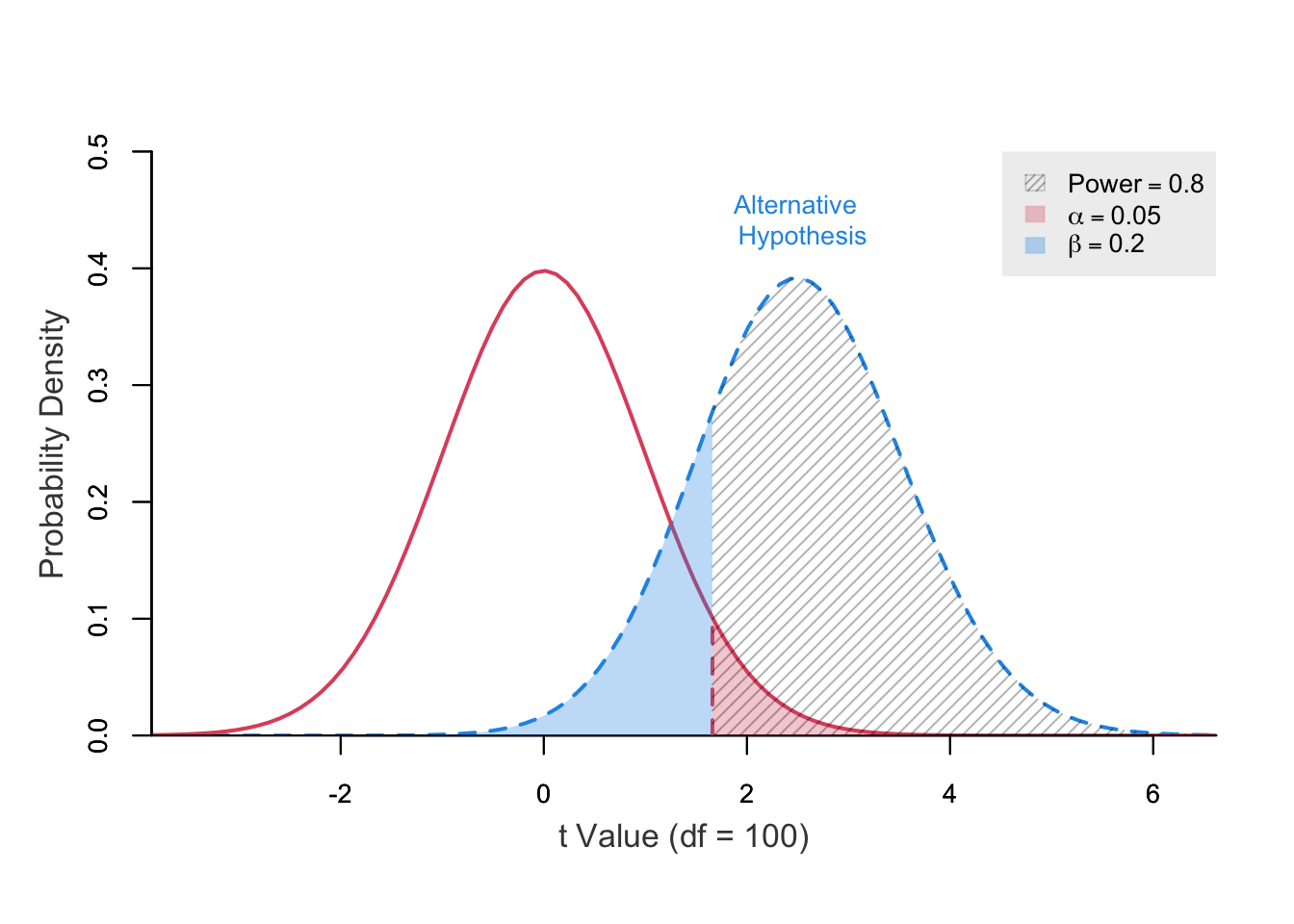
These functions compute statistical power and can plot Type I and II errors if test statistics and degrees of freedom are known.
They’re useful because z, t, $\chi^{2}$, and F stats with degrees of freedom are often reported in publications or software outputs.
Power can be calculated from test statistics as noncentrality parameters, but post-hoc power estimates should be interpreted cautiously.

t Test

power.t.test(ncp = 1.96, df = 99, alpha = 0.05,
             alternative = "equivalent", plot = TRUE)

t Test

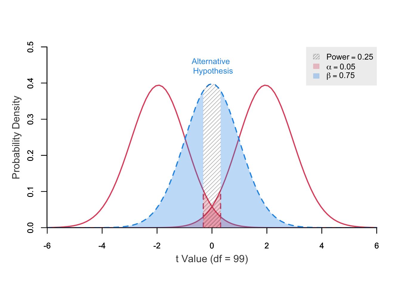
     power ncp.alt ncp.null.1 ncp.null.2 alpha df   t.crit.1  t.crit.2
 0.2371389       0      -1.96       1.96  0.05 99 -0.3155295 0.3155295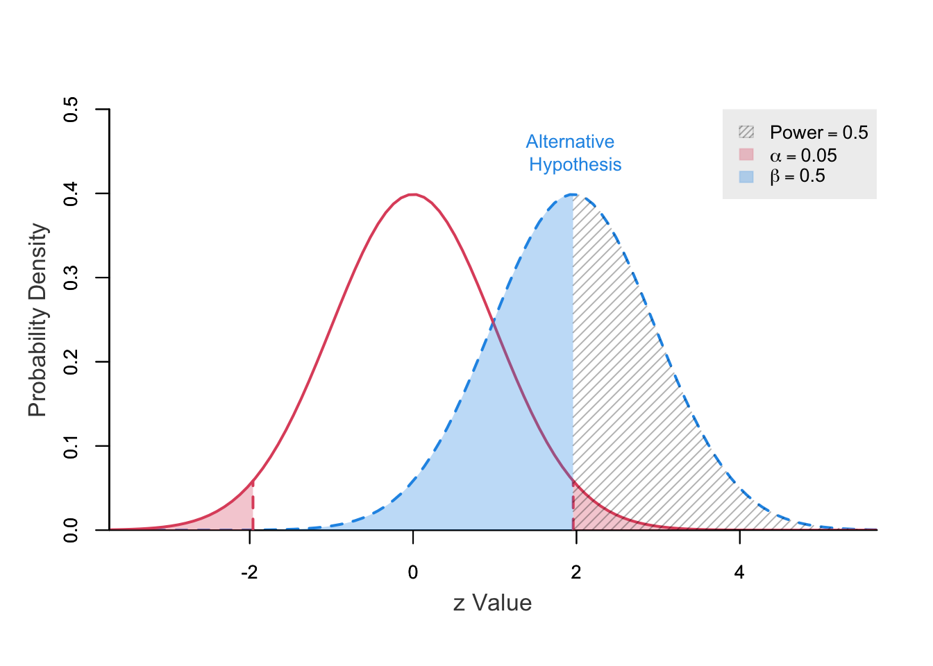

z Test

power.z.test(ncp = 1.96, alpha = 0.05, 
             alternative = "not equal", plot = TRUE)

z Test

     power ncp.alt ncp.null alpha  z.crit.1 z.crit.2
 0.5000586    1.96        0  0.05 -1.959964 1.959964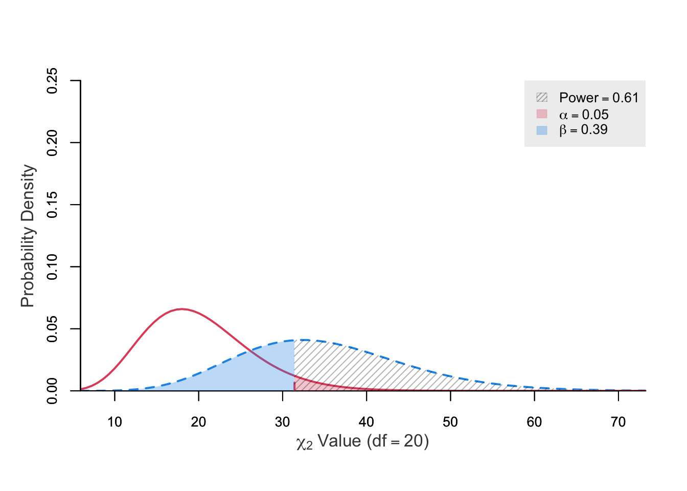

$\chi^2$ Test

power.chisq.test(ncp = 15, df = 20,
                 alpha = 0.05, plot = TRUE)

$\chi^2$ Test

     power ncp.alt ncp.null alpha df chisq.crit
 0.6110368      15        0  0.05 20   31.41043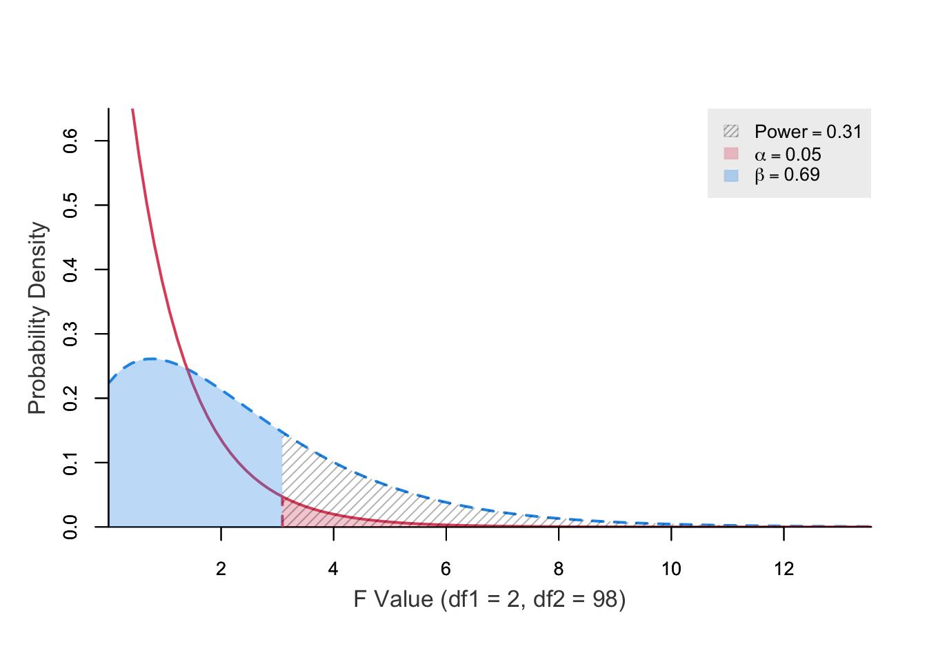

F Test

power.f.test(ncp = 3, df1 = 2, df2 = 98,
             alpha = 0.05, plot = TRUE)

F Test

     power ncp.alt ncp.null alpha df1 df2   f.crit
 0.3128778       3        0  0.05   2  98 3.089203

Multiple Parameters

Multiple parameters are allowed but plots should be turned off (plot = FALSE).

t Test

power.t.test(
  ncp = c(0.50, 1.00, 1.50, 2.00, 2.50), 
  plot = FALSE,
  df = 99, 
  alpha = 0.05, 
  alternative = "not equal")

t Test

      power ncp.alt ncp.null alpha df  t.crit.1 t.crit.2
 0.07852973     0.5        0  0.05 99 -1.984217 1.984217
 0.16769955     1.0        0  0.05 99 -1.984217 1.984217
 0.31785490     1.5        0  0.05 99 -1.984217 1.984217
 0.50826481     2.0        0  0.05 99 -1.984217 1.984217
 0.69698027     2.5        0  0.05 99 -1.984217 1.984217

z Test

power.z.test(
  alpha = c(0.001, 0.010, 0.025, 0.050), 
  plot = FALSE,
  ncp = 1.96, 
  alternative = "greater")

z Test

     power ncp.alt ncp.null alpha   z.crit
 0.1291892    1.96        0 0.001 3.090232
 0.3570528    1.96        0 0.010 2.326348
 0.5000144    1.96        0 0.025 1.959964
 0.6236747    1.96        0 0.050 1.644854

$\chi^2$ Test

power.chisq.test(
  df = c(80, 90, 100, 120, 150, 200), 
  plot = FALSE, 
  ncp = 2, 
  alpha = 0.05)

$\chi^2$ Test

      power ncp.alt ncp.null alpha  df chisq.crit
 0.06989507       2        0  0.05  80   101.8795
 0.06856779       2        0  0.05  90   113.1453
 0.06746196       2        0  0.05 100   124.3421
 0.06571411       2        0  0.05 120   146.5674
 0.06382959       2        0  0.05 150   179.5806
 0.06175379       2        0  0.05 200   233.9943

Type I and Type II Error Plots

We use the plot() function (S3 method) is a wrapper around the generic functions above. Assign results of any pwrss function to an R object and pass it to plot() function.

Comparing two means

design1 <- pwrss.t.2means(
  mu1 = 0.20, 
  margin = -0.05, 
  paired = TRUE,
  power = 0.80, 
  alpha = 0.05,
  alternative = "non-inferior")

Comparing two means

 Difference between Two means 
 (Paired Samples t Test) 
 H0: mu1 - mu2 <= margin 
 HA: mu1 - mu2 > margin 
 ------------------------------ 
  Statistical power = 0.8 
  n = 101 
 ------------------------------ 
 Alternative = "non-inferior" 
 Degrees of freedom = 100 
 Non-centrality parameter = 2.512 
 Type I error rate = 0.05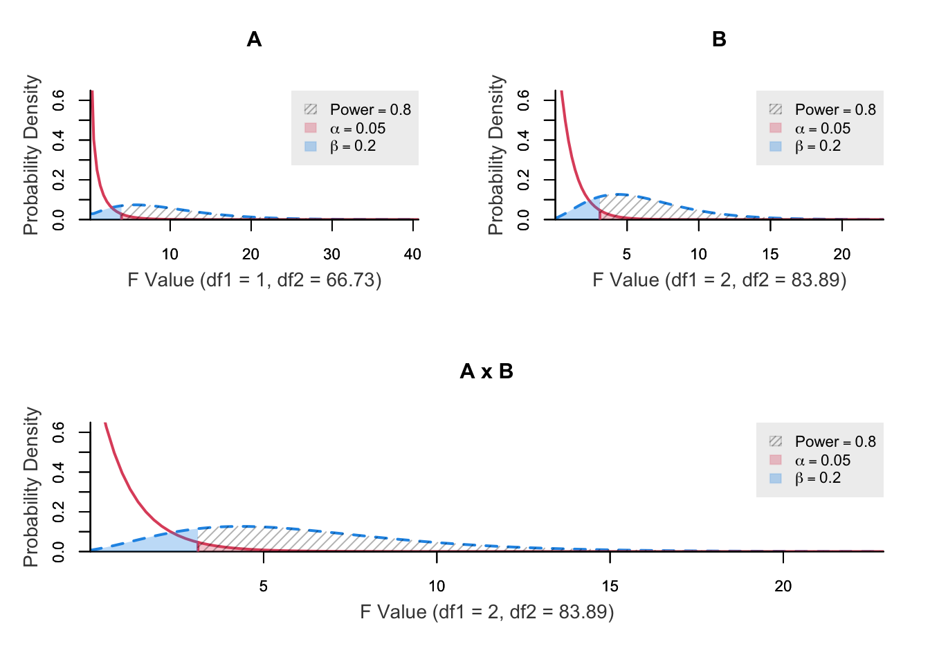 
 Type II error rate = 0.2

Comparing two means

plot(design1)

ANCOVA

design3 <- pwrss.f.ancova(
  eta2 = 0.10, 
  n.levels = c(2,3),
  power = .80, 
  alpha = 0.05)

ANCOVA

 Two-way Analysis of Variance (ANOVA) 
  H0: 'eta2' or 'f2' = 0 
  HA: 'eta2' or 'f2' > 0 
 --------------------------------------
 Factor A: 2 levels 
 Factor B: 3 levels 
 --------------------------------------
 effect power n.total   ncp df1    df2
      A   0.8      73 8.081   1 66.729
      B   0.8      90 9.987   2 83.885
  A x B   0.8      90 9.987   2 83.885
 --------------------------------------
 Type I error rate: 0.05

ANCOVA

plot(design3)

Mean Difference (t Tests) Parametric Tests

Independent Samples t Test

More often than not, unstandardized means and standard deviations are reported in publications for descriptive purposes. Another reason is that they are more intuitive and interpretable (e.g. depression scale). Assume that for the first and second groups expected means are 30 and 28, and expected standard deviations are 12 and 8, respectively.

Calculate Statistical Power

What is the statistical power given that the sample size for the second group is 50 (n2 = 50) and groups have equal sample sizes (kappa = n1 / n2 = 1)?

pwrss.t.2means(mu1 = 30, mu2 = 28, sd1 = 12, sd2 = 8, kappa = 1, 
               n2 = 50, alpha = 0.05,
               alternative = "not equal")

Calculate Statistical Power

 Difference between Two means 
 (Independent Samples t Test) 
 H0: mu1 = mu2 
 HA: mu1 != mu2 
 ------------------------------ 
  Statistical power = 0.163 
  n1 = 50 
  n2 = 50 
 ------------------------------ 
 Alternative = "not equal" 
 Degrees of freedom = 98 
 Non-centrality parameter = 0.981 
 Type I error rate = 0.05 
 Type II error rate = 0.837

Calculate Minimum Required Sample Size

What is the minimum required sample size given that groups have equal sample sizes (kappa = 1)? ($\kappa = n_1 / n_2$)

pwrss.t.2means(mu1 = 30, mu2 = 28, sd1 = 12, sd2 = 8, kappa = 1, 
               power = .80, alpha = 0.05,
               alternative = "not equal")

Calculate Minimum Required Sample Size

 Difference between Two means 
 (Independent Samples t Test) 
 H0: mu1 = mu2 
 HA: mu1 != mu2 
 ------------------------------ 
  Statistical power = 0.8 
  n1 = 410 
  n2 = 410 
 ------------------------------ 
 Alternative = "not equal" 
 Degrees of freedom = 818 
 Non-centrality parameter = 2.808 
 Type I error rate = 0.05 
 Type II error rate = 0.2

Calculate Minimum Required Sample Size

It is sufficient to put pooled standard deviation for sd1 because sd2 = sd1 by default. In this case, for a pooled standard deviation of 10.198 the minimum required sample size can be calculated as

pwrss.t.2means(mu1 = 30, mu2 = 28, sd1 = 10.198, kappa = 1,
               power = .80, alpha = 0.05,
               alternative = "not equal")

Calculate Minimum Required Sample Size

 Difference between Two means 
 (Independent Samples t Test) 
 H0: mu1 = mu2 
 HA: mu1 != mu2 
 ------------------------------ 
  Statistical power = 0.8 
  n1 = 410 
  n2 = 410 
 ------------------------------ 
 Alternative = "not equal" 
 Degrees of freedom = 818 
 Non-centrality parameter = 2.808 
 Type I error rate = 0.05 
 Type II error rate = 0.2

Calculate Minimum Required Sample Size

It is sufficient to put Cohen’s d or Hedge’s g (standardized difference between two groups) for mu1 because mu2 = 0, sd1 = 1, and sd2 = sd1 by default. For example, for an effect size as small as 0.196 (based on previous example) the minimum required sample size can be calculated as

pwrss.t.2means(mu1 = 0.196, kappa = 1,
               power = .80, alpha = 0.05, 
               alternative = "not equal")

Calculate Minimum Required Sample Size

 Difference between Two means 
 (Independent Samples t Test) 
 H0: mu1 = mu2 
 HA: mu1 != mu2 
 ------------------------------ 
  Statistical power = 0.8 
  n1 = 410 
  n2 = 410 
 ------------------------------ 
 Alternative = "not equal" 
 Degrees of freedom = 818 
 Non-centrality parameter = 2.806 
 Type I error rate = 0.05 
 Type II error rate = 0.2

Paired Samples t Test

Assume for the first (e.g. pretest) and second (e.g. posttest) time points expected means are 30 and 28 (a reduction of 2 points), and expected standard deviations are 12 and 8, respectively. Also assume a correlation of 0.50 between first and second measurements (by default paired.r = 0.50). What is the minimum required sample size?

pwrss.t.2means(mu1 = 30, mu2 = 28, sd1 = 12, sd2 = 8, 
               paired = TRUE, paired.r = 0.50,
               power = .80, alpha = 0.05,
               alternative = "not equal")

Paired Samples t Test

 Difference between Two means 
 (Paired Samples t Test) 
 H0: mu1 = mu2 
 HA: mu1 != mu2 
 ------------------------------ 
  Statistical power = 0.8 
  n = 222 
 ------------------------------ 
 Alternative = "not equal" 
 Degrees of freedom = 221 
 Non-centrality parameter = 2.816 
 Type I error rate = 0.05 
 Type II error rate = 0.2

Calculate Minimum Required Sample Size

It is sufficient to put standard deviation of the difference for sd1 because sd2 = sd1 by default. In this case, for a standard deviation of difference of 10.583 the minimum required sample size can be calculated as

pwrss.t.2means(mu1 = 30, mu2 = 28, sd1 = 10.583, 
               paired = TRUE, paired.r = 0.50,
               power = .80, alpha = 0.05,
               alternative = "not equal")

Calculate Minimum Required Sample Size

 Difference between Two means 
 (Paired Samples t Test) 
 H0: mu1 = mu2 
 HA: mu1 != mu2 
 ------------------------------ 
  Statistical power = 0.8 
  n = 222 
 ------------------------------ 
 Alternative = "not equal" 
 Degrees of freedom = 221 
 Non-centrality parameter = 2.816 
 Type I error rate = 0.05 
 Type II error rate = 0.2

Calculate Minimum Required Sample Size

It is sufficient to put Cohen’s d or Hedge’s g (standardized difference between two time points) for mu1 because mu2 = 0, sd1 = sqrt(1/(2*(1-paired.r))), and sd2 = sd1 by default. For example, for an effect size as small as 0.1883 (based on previous example) the minimum required sample size can be calculated as

pwrss.t.2means(mu1 = 0.1883, paired = TRUE, paired.r = 0.50,
               power = .80, alpha = 0.05, 
               alternative = "not equal")

Calculate Minimum Required Sample Size

 Difference between Two means 
 (Paired Samples t Test) 
 H0: mu1 = mu2 
 HA: mu1 != mu2 
 ------------------------------ 
  Statistical power = 0.8 
  n = 224 
 ------------------------------ 
 Alternative = "not equal" 
 Degrees of freedom = 223 
 Non-centrality parameter = 2.818 
 Type I error rate = 0.05 
 Type II error rate = 0.2

Non-parametric Tests

Means might be compared for variables that aren’t normally distributed, due to small samples or inherently non-normal population distributions (e.g. uniform, exponential).
In such cases, t-tests may give biased results.
For non-parametric tests, use pwrss.np.2groups() instead of pwrss.t.2means(), with the same arguments.

Non-parametric Tests

You can specify the parent distribution (e.g. "normal", "uniform", "exponential") using the dist argument.

Although the function uses means and standard deviations as inputs, it actually tests differences in mean ranks.
Mean differences are converted to Cohen’s d and then to probability of superiority, making it easier to compare and switch between parametric and non-parametric tests.

Independent Samples (Wilcoxon-Mann-Whitney Test)

The example below uses the same parameters as the example in the independent t test section.

pwrss.np.2groups(mu1 = 30, mu2 = 28, sd1 = 12, sd2 = 8, kappa = 1, 
               power = .80, alpha = 0.05,
               alternative = "not equal")

Independent Samples (Wilcoxon-Mann-Whitney Test)

 Non-parametric Difference between Two Groups (Independent samples) 
 Mann-Whitney U or Wilcoxon Rank-sum Test 
 (a.k.a Wilcoxon-Mann-Whitney Test) 
 Method: GUENTHER 
 ------------------------------ 
  Statistical power = 0.8 
  n1 = 429 
  n2 = 429 
 ------------------------------ 
 Alternative = "not equal" 
 Non-centrality parameter = 2.805 
 Degrees of freedom = 816.21 
 Type I error rate = 0.05 
 Type II error rate = 0.2

Paired Samples (Wilcoxon Signed-rank Test)

The example below uses the same parameters as the example in the paired (dependent) t test section.

pwrss.np.2groups(mu1 = 30, mu2 = 28, sd1 = 12, sd2 = 8, 
               paired = TRUE, paired.r = 0.50,
               power = .80, alpha = 0.05,
               alternative = "not equal")

It is sufficient to put Cohen’s d or Hedge’s g (standardized difference between two groups or measurements) for mu1 without specifying mu2, sd1, and sd2.

Paired Samples (Wilcoxon Signed-rank Test)

 Non-parametric Difference between Two Groups (Dependent samples) 
 Wilcoxon signed-rank Test for Matched Pairs 
 Method: GUENTHER 
 ------------------------------ 
  Statistical power = 0.8 
  n = 233 
 ------------------------------ 
 Alternative = "not equal" 
 Non-centrality parameter = 2.814 
 Degrees of freedom = 220.7 
 Type I error rate = 0.05 
 Type II error rate = 0.2

Non-inferiority, Superiority, and Equivalence

These tests are useful for testing practically significant difference (non-inferiority/superiority) or practically null difference (equivalence).

Parametric Tests

Non-inferiority: The mean of group 1 is practically not smaller than the mean of group 2. The mu1 - mu2 difference can be as small as -1 (margin = -1) but it will still be considered non-inferior. What is the minimum required sample size?

Parametric Tests

When higher values of an outcome is better the margin takes NEGATIVE values; whereas when lower values of the outcome is better margin takes POSITIVE values.

pwrss.t.2means(mu1 = 30, mu2 = 28, sd1 = 12, sd2 = 8, 
               margin = -1, power = 0.80,
               alternative = "non-inferior")

Parametric Tests

 Difference between Two means 
 (Independent Samples t Test) 
 H0: mu1 - mu2 <= margin 
 HA: mu1 - mu2 > margin 
 ------------------------------ 
  Statistical power = 0.8 
  n1 = 144 
  n2 = 144 
 ------------------------------ 
 Alternative = "non-inferior" 
 Degrees of freedom = 286 
 Non-centrality parameter = 2.496 
 Type I error rate = 0.05 
 Type II error rate = 0.2

Parametric Tests

Superiority: The mean of group 1 is practically greater than the mean of group 2. The mu1 - mu2 difference is at least greater than 1 (margin = 1). What is the minimum required sample size?

When higher values of an outcome is better margin takes POSITIVE values; whereas when lower values of the outcome is better margin takes NEGATIVE values.

pwrss.t.2means(mu1 = 30, mu2 = 28, sd1 = 12, sd2 = 8, 
               margin = 1, power = 0.80,
               alternative = "superior")

Parametric Tests

 Difference between Two means 
 (Independent Samples t Test) 
 H0: mu1 - mu2 <= margin 
 HA: mu1 - mu2 > margin 
 ------------------------------ 
  Statistical power = 0.8 
  n1 = 1287 
  n2 = 1287 
 ------------------------------ 
 Alternative = "superior" 
 Degrees of freedom = 2572 
 Non-centrality parameter = 2.487 
 Type I error rate = 0.05 
 Type II error rate = 0.2

Parametric Tests

Equivalence: The mean of group 1 is practically same as mean of group 2. The mu1 - mu2 difference can be as small as -1 and as high as 1 (margin = 1). What is the minimum required sample size?

Specify the absolute value for the margin.

pwrss.t.2means(mu1 = 30, mu2 = 30, sd1 = 12, sd2 = 8, 
               margin = 1, power = 0.80,
               alternative = "equivalent")

Parametric Tests

 Difference between Two means 
 (Independent Samples t Test) 
 H0: |mu1 - mu2| >= margin 
 HA: |mu1 - mu2| < margin 
 ------------------------------ 
  Statistical power = 0.8 
  n1 = 1783 
  n2 = 1783 
 ------------------------------ 
 Alternative = "equivalent" 
 Degrees of freedom = 3564 
 Non-centrality parameter = -2.928 
 Type I error rate = 0.05 
 Type II error rate = 0.2

Non-parametric Tests

Non-inferiority: The mean of group 1 is practically not smaller than the mean of group 2. The mu1 - mu2 difference can be as small as -1 (margin = -1). What is the minimum required sample size?

pwrss.np.2groups(mu1 = 30, mu2 = 28, sd1 = 12, sd2 = 8, 
               margin = -1, power = 0.80,
               alternative = "non-inferior")

Non-parametric Tests

 Non-parametric Difference between Two Groups (Independent samples) 
 Mann-Whitney U or Wilcoxon Rank-sum Test 
 (a.k.a Wilcoxon-Mann-Whitney Test) 
 Method: GUENTHER 
 ------------------------------ 
  Statistical power = 0.8 
  n1 = 151 
  n2 = 151 
 ------------------------------ 
 Alternative = "non-inferior" 
 Non-centrality parameter = 2.492 
 Degrees of freedom = 285.13 
 Type I error rate = 0.05 
 Type II error rate = 0.2

Non-parametric Tests

Superiority: The mean of group 1 is practically greater than the mean of group 2. The mu1 - mu2 difference is at least greater than 1 (margin = 1). What is the minimum required sample size?

pwrss.np.2groups(mu1 = 30, mu2 = 28, sd1 = 12, sd2 = 8, 
               margin = 1, power = 0.80,
               alternative = "superior")

Non-parametric Tests

 Non-parametric Difference between Two Groups (Independent samples) 
 Mann-Whitney U or Wilcoxon Rank-sum Test 
 (a.k.a Wilcoxon-Mann-Whitney Test) 
 Method: GUENTHER 
 ------------------------------ 
  Statistical power = 0.8 
  n1 = 1348 
  n2 = 1348 
 ------------------------------ 
 Alternative = "superior" 
 Non-centrality parameter = 2.487 
 Degrees of freedom = 2571.3 
 Type I error rate = 0.05 
 Type II error rate = 0.2

Non-parametric Tests

pwrss.np.2groups(mu1 = 30, mu2 = 30, sd1 = 12, sd2 = 8, 
               margin = 1, power = 0.80,
               alternative = "equivalent")

Non-parametric Tests

 Non-parametric Difference between Two Groups (Independent samples) 
 Mann-Whitney U or Wilcoxon Rank-sum Test 
 (a.k.a Wilcoxon-Mann-Whitney Test) 
 Method: GUENTHER 
 ------------------------------ 
  Statistical power = 0.8 
  n1 = 1867 
  n2 = 1867 
 ------------------------------ 
 Alternative = "equivalent" 
 Non-centrality parameter = -2.927 
 Degrees of freedom = 3561.91 
 Type I error rate = 0.05 
 Type II error rate = 0.2

Linear Regression (F and t Tests)

Omnibus $F$ Test

$R^2 > 0$ in Linear Regression

Omnibus F test in multiple liner regression is used to test whether $R^2$ is greater than 0 (zero). Assume that we want to predict a continuous variable $Y$ using $X_{1}$, $X_{2}$, and $X_{2}$ variables (a combination of binary or continuous).

\[\begin{eqnarray} Y &=& \beta_{0} + \beta_{1}X_{1} + \beta_{2}X_{2} + \beta_{3}X_{3} + r, \quad r \thicksim N(0,\sigma^2) \newline \end{eqnarray}\]

Linear Regression (F and t Tests)

We are expecting that these three variables explain 30% of the variance in the outcome ($R^2 = 0.30$ or r2 = 0.30 in the code). What is the minimum required sample size?

pwrss.f.reg(r2 = 0.30, k = 3, power = 0.80, alpha = 0.05)

Linear Regression (F and t Tests)

 Linear Regression (F test) 
 R-squared Deviation from 0 (zero) 
 H0: r2 = 0 
 HA: r2 > 0 
 ------------------------------ 
  Statistical power = 0.8 
  n = 30 
 ------------------------------ 
 Numerator degrees of freedom = 3 
 Denominator degrees of freedom = 25.653 
 Non-centrality parameter = 12.709 
 Type I error rate = 0.05 
 Type II error rate = 0.2

Single Regression Coefficient (z or t Test)

Standardized versus Unstandardized Input

In the earlier example, assume that we want to predict a continuous variable $Y$ using a continuous predictor $X_{1}$ but control for $X_{2}$, and $X_{2}$ variables (a combination of binary or continuous). We are mainly interested in the effect of $X_{1}$ and expect a standardized regression coefficient of $\beta_{1} = 0.20$.

\[\begin{eqnarray} Y &=& \beta_{0} + \color{red} {\beta_{1} X_{1}} + \beta_{2}X_{2} + \beta_{3}X_{3} + r, \quad r \thicksim N(0,\sigma^2) \newline \end{eqnarray}\]

Single Regression Coefficient (z or t Test)

Again, we are expecting that these three variables explain 30% of the variance in the outcome ($R^2 = 0.30$). What is the minimum required sample size? It is sufficient to provide standardized regression coefficient for beta1 because sdx = 1 and sdy = 1 by default.

pwrss.t.reg(beta1 = 0.20, k = 3, r2 = 0.30, 
            power = .80, alpha = 0.05, alternative = "not equal")

Single Regression Coefficient (z or t Test)

 Linear Regression Coefficient (t Test) 
 H0: beta1 = beta0 
 HA: beta1 != beta0 
 ------------------------------ 
  Statistical power = 0.8 
  n = 140 
 ------------------------------ 
 Alternative = "not equal" 
 Degrees of freedom = 135.331 
 Non-centrality parameter = 2.822 
 Type I error rate = 0.05 
 Type II error rate = 0.2

Single Regression Coefficient (z or t Test)

For unstandardized coefficients specify sdy and sdx. Assume we are expecting an unstandardized regression coefficient of beta1 = 0.60, a standard deviation of sdy = 12 for the outcome and a standard deviation of sdx = 4 for the main predictor. What is the minimum required sample size?

pwrss.t.reg(beta1 = 0.60, sdy = 12, sdx = 4, k = 3, r2 = 0.30, 
            power = .80, alpha = 0.05, alternative = "not equal")

Single Regression Coefficient (z or t Test)

 Linear Regression Coefficient (t Test) 
 H0: beta1 = beta0 
 HA: beta1 != beta0 
 ------------------------------ 
  Statistical power = 0.8 
  n = 140 
 ------------------------------ 
 Alternative = "not equal" 
 Degrees of freedom = 135.331 
 Non-centrality parameter = 2.822 
 Type I error rate = 0.05 
 Type II error rate = 0.2

Single Regression Coefficient (z or t Test)

When the main predictor is binary (e.g. treatment/control), its standardized regression coefficient equals Cohen’s d.
The predictor’s standard deviation is $\sqrt{p(1-p)}$, where $p$ is the group proportion; for $p = 0.50$, what’s the minimum required sample size?
Provide Cohen’s d for β₁ and set sdx = sqrt(p*(1-p)) when calculating.

p <- 0.50
pwrss.t.reg(beta1 = 0.20, k = 3, r2 = 0.30, sdx = sqrt(p*(1-p)),
            power = .80, alpha = 0.05, alternative = "not equal")

Single Regression Coefficient (z or t Test)

 Linear Regression Coefficient (t Test) 
 H0: beta1 = beta0 
 HA: beta1 != beta0 
 ------------------------------ 
  Statistical power = 0.8 
  n = 552 
 ------------------------------ 
 Alternative = "not equal" 
 Degrees of freedom = 547.355 
 Non-centrality parameter = 2.807 
 Type I error rate = 0.05 
 Type II error rate = 0.2

Non-inferiority, Superiority, and Equivalence

These tests are useful for testing practically significant effects (non-inferiority/superiority) or practically null effects (equivalence).

Non-inferiority:

The intervention is expected to be non-inferior to some earlier or other interventions. Assume that the effect of an earlier or some other intervention is beta0 = 0.10. The beta1 - beta0 is expected to be positive and should be at least -0.05 (margin = -0.05). What is the minimum required sample size?

Non-inferiority:

This is the case when higher values of an outcome is better. When lower values of an outcome is better the beta1 - beta0 difference is expected to be NEGATIVE and the margin takes POSITIVE values.

p <- 0.50
pwrss.t.reg(beta1 = 0.20, beta0 = 0.10, margin = -0.05, 
            k = 3, r2 = 0.30, sdx = sqrt(p*(1-p)),
            power = .80, alpha = 0.05, alternative = "non-inferior")

Non-inferiority:

 Linear Regression Coefficient (t Test) 
 H0: beta1 - beta0 <= margin 
 HA: beta1 - beta0 > margin 
 ------------------------------ 
  Statistical power = 0.8 
  n = 771 
 ------------------------------ 
 Alternative = "non-inferior" 
 Degrees of freedom = 766.745 
 Non-centrality parameter = 2.489 
 Type I error rate = 0.05 
 Type II error rate = 0.2

Superiority

The intervention is expected to be superior to some earlier or other interventions. Assume that the effect of an earlier or some other intervention is beta0 = 0.10. The beta1 - beta0 is expected to be positive and should be at least 0.05 (margin = 0.05). What is the minimum required sample size?

Superiority

This is the case when higher values of an outcome is better. When lower values of an outcome is better beta1 - beta0 difference is expected to be NEGATIVE and the margin takes NEGATIVE values.

p <- 0.50
pwrss.t.reg(beta1 = 0.20, beta0 = 0.10, margin = 0.05, 
            k = 3, r2 = 0.30, sdx = sqrt(p*(1-p)),
            power = .80, alpha = 0.05, alternative = "superior")

Superiority

 Linear Regression Coefficient (t Test) 
 H0: beta1 - beta0 <= margin 
 HA: beta1 - beta0 > margin 
 ------------------------------ 
  Statistical power = 0.8 
  n = 6926 
 ------------------------------ 
 Alternative = "superior" 
 Degrees of freedom = 6921.818 
 Non-centrality parameter = 2.487 
 Type I error rate = 0.05 
 Type II error rate = 0.2

Equivalence

The intervention is expected to be equivalent to some earlier or other interventions. Assume the effect of an earlier or some other intervention is beta0 = 0.20. The beta1 - beta0 is expected to be within -0.05 and 0.05 (margin = 0.05). What is the minimum required sample size?

Equivalence

margin always takes positive values for equivalence. Specify the absolute value.

p <- 0.50
pwrss.t.reg(beta1 = 0.20, beta0 = 0.20, margin = 0.05, 
            k = 3, r2 = 0.30, sdx = sqrt(p*(1-p)),
            power = .80, alpha = 0.05, alternative = "equivalent")

Equivalence

 Linear Regression Coefficient (t Test) 
 H0: |beta1 - beta0| >= margin 
 HA: |beta1 - beta0| < margin 
 ------------------------------ 
  Statistical power = 0.8 
  n = 9593 
 ------------------------------ 
 Alternative = "equivalent" 
 Degrees of freedom = 9588.862 
 Non-centrality parameter = -2.927 2.927 
 Type I error rate = 0.05 
 Type II error rate = 0.2

Logistic Regression (Wald’s z Test)

In logistic regression a binary outcome variable (0/1: failed/passed, dead/alive, absent/present) is modeled by predicting probability of being in group 1 ($P_1$) via logit transformation (natural logarithm of odds). The base probability $P_0$ is the overall probability of being in group 1 without influence of predictors in the model (null). Under alternative hypothesis, the probability of being in group 1 ($P_1$) deviate from $P_0$ depending on the value of the predictor; whereas under null it is same as the $P_0$.

Logistic Regression (Wald’s z Test)

A model with one main predictor ($X_1$) and two other covariates ($X_2$ and $X_3$) can be constructed as

\[\begin{eqnarray} ln(\frac{P_1}{1- P_1}) &=& \beta_{0} + \color{red} {\beta_{1} X_{1}} + \beta_{2}X_{2} + \beta_{3}X_{3} \newline \end{eqnarray}\]

Logistic Regression (Wald’s z Test)

Therefore the odds ratio is defined as \[OR = exp(\beta_1) = \frac{P_1}{1- P_1} / \frac{P_0}{1- P_0}\]

Logistic Regression (Wald’s z Test)

Example:

A squared multiple correlation of 0.20 between $X_1$ and other covariates (r2.other.x = 0.20 in the code). It can be found in the form of adjusted R-square via regressing $X_1$ on $X_2$ and $X_3$. Higher values require larger sample sizes. The default is 0 (zero).
A base probability of $P_0 = 0.15$. This is the rate when predictor $X_1 = 0$ or when $\beta_1 = 0$.
Increasing $X_1$ from 0 to 1 reduces the probability of being in group 1 from 0.15 to 0.10 ($P_1 = 0.10$).

Logistic Regression (Wald’s z Test)

What is the minimum required sample size? There are three types of specification to statistical power or sample size calculations; (i) probability specification, (ii) odds ratio specification, and (iii) regression coefficient specification (as in standard software output).

Logistic Regression (Wald’s z Test)

Probability specification:

pwrss.z.logreg(p0 = 0.15, p1 = 0.10, r2.other.x = 0.20,
               power = 0.80, alpha = 0.05, 
               dist = "normal")

Logistic Regression (Wald’s z Test)

 Logistic Regression Coefficient 
 (Large Sample Approx. Wald's z Test) 
 H0: beta1 = 0 
 HA: beta1 != 0 
 Distribution of X = 'normal' 
 Method = DEMIDENKO(VC) 
 ------------------------------ 
  Statistical power = 0.8 
  n = 365 
 ------------------------------ 
 Alternative = "not equal" 
 Non-centrality parameter = -2.766 
 Type I error rate = 0.05 
 Type II error rate = 0.2

Logistic Regression (Wald’s z Test)

Odds ratio specification: \[OR = \frac{P_1}{1-P1} / \frac{P_0}{1-P_0} = \frac{0.10}{1-0.10} / \frac{0.15}{1-0.15} = 0.6296\]

pwrss.z.logreg(p0 = 0.15, odds.ratio = 0.6296, r2.other.x = 0.20,
               alpha = 0.05, power = 0.80,
               dist = "normal")

Logistic Regression (Wald’s z Test)

 Logistic Regression Coefficient 
 (Large Sample Approx. Wald's z Test) 
 H0: beta1 = 0 
 HA: beta1 != 0 
 Distribution of X = 'normal' 
 Method = DEMIDENKO(VC) 
 ------------------------------ 
  Statistical power = 0.8 
  n = 365 
 ------------------------------ 
 Alternative = "not equal" 
 Non-centrality parameter = -2.766 
 Type I error rate = 0.05 
 Type II error rate = 0.2

Logistic Regression (Wald’s z Test)

Regression coefficient specification: \[\beta_1 = ln(\frac{P_1}{1-P1} / \frac{P_0}{1-P_0}) = ln(0.6296) = -0.4626\]

pwrss.z.logreg(p0 = 0.15, beta1 = -0.4626, r2.other.x = 0.20,
               alpha = 0.05, power = 0.80,
               dist = "normal")

Logistic Regression (Wald’s z Test)

 Logistic Regression Coefficient 
 (Large Sample Approx. Wald's z Test) 
 H0: beta1 = 0 
 HA: beta1 != 0 
 Distribution of X = 'normal' 
 Method = DEMIDENKO(VC) 
 ------------------------------ 
  Statistical power = 0.8 
  n = 365 
 ------------------------------ 
 Alternative = "not equal" 
 Non-centrality parameter = -2.766 
 Type I error rate = 0.05 
 Type II error rate = 0.2

Logistic Regression (Wald’s z Test)

Change the distribution’s parameters for predictor X:

The mean and standard deviation of a normally distributed main predictor is 0 and 1 by default. They can be modified. In the following example the mean is 25 and the standard deviation is 8.

dist.x <- list(dist = "normal", mean = 25, sd = 8)

pwrss.z.logreg(p0 = 0.15, beta1 = -0.4626, r2.other.x = 0.20,
               alpha = 0.05, power = 0.80,
               dist = dist.x)

Logistic Regression (Wald’s z Test)

 Logistic Regression Coefficient 
 (Large Sample Approx. Wald's z Test) 
 H0: beta1 = 0 
 HA: beta1 != 0 
 Distribution of X = 'normal' 
 Method = DEMIDENKO(VC) 
 ------------------------------ 
  Statistical power = 0.8 
  n = 2435 
 ------------------------------ 
 Alternative = "not equal" 
 Non-centrality parameter = -2.423 
 Type I error rate = 0.05 
 Type II error rate = 0.2

Logistic Regression (Wald’s z Test)

Change the distribution family of predictor X:

More distribution types are supported by the function. For example, the main predictor can be binary (e.g. treatment/control groups). Often half of the sample is assigned to the treatment group and the other half to the control (prob = 0.50 by default).

pwrss.z.logreg(p0 = 0.15, beta1 = -0.4626, r2.other.x = 0.20,
               alpha = 0.05, power = 0.80,
               dist = "bernoulli")

Logistic Regression (Wald’s z Test)

 Logistic Regression Coefficient 
 (Large Sample Approx. Wald's z Test) 
 H0: beta1 = 0 
 HA: beta1 != 0 
 Distribution of X = 'bernoulli' 
 Method = DEMIDENKO(VC) 
 ------------------------------ 
  Statistical power = 0.8 
  n = 1723 
 ------------------------------ 
 Alternative = "not equal" 
 Non-centrality parameter = -2.789 
 Type I error rate = 0.05 
 Type II error rate = 0.2

Logistic Regression (Wald’s z Test)

Change the treatment group allocation rate of the binary predictor X (prob = 0.40):

Sometimes treatment groups cost more per subject or are harder to recruit than control groups, making an unbalanced sample practical. For example, with 40% of subjects in the treatment group, what is the minimum required sample size?

dist.x <- list(dist = "bernoulli", prob = 0.40)

pwrss.z.logreg(p0 = 0.15, beta1 = -0.4626, r2.other.x = 0.20,
               alpha = 0.05, power = 0.80,
               dist = dist.x)

Logistic Regression (Wald’s z Test)

 Logistic Regression Coefficient 
 (Large Sample Approx. Wald's z Test) 
 H0: beta1 = 0 
 HA: beta1 != 0 
 Distribution of X = 'bernoulli' 
 Method = DEMIDENKO(VC) 
 ------------------------------ 
  Statistical power = 0.8 
  n = 1826 
 ------------------------------ 
 Alternative = "not equal" 
 Non-centrality parameter = -2.766 
 Type I error rate = 0.05 
 Type II error rate = 0.2

Analysis of (Co)Variance (F Test)

ANOVA: Analysis of Variance ANCOVA: Analysis of Covariance

One-way ANOVA/ANCOVA: Compares means across groups; ANCOVA adjusts for covariates.
Two- or Three-way ANOVA/ANCOVA: Examines interactions between factors; ANCOVA adjusts interactions for covariates and determines required sample size for complex designs.

One-way

ANOVA

A researcher is expecting a difference of Cohen’s d = 0.50 between treatment and control groups (two levels) translating into $\eta^2 = 0.059$ (eta2 = 0.059). Means are not adjusted for any covariates. What is the minimum required sample size?

pwrss.f.ancova(eta2 = 0.059, n.levels = 2,
               power = .80, alpha = 0.05)

One-way

 One-way Analysis of Variance (ANOVA) 
  H0: 'eta2' or 'f2' = 0 
  HA: 'eta2' or 'f2' > 0 
 --------------------------------------
 Factor A: 2 levels 
 --------------------------------------
 effect power n.total   ncp df1     df2
      A   0.8     128 7.971   1 125.132
 --------------------------------------
 Type I error rate: 0.05

One-way

ANCOVA

A researcher is expecting an adjusted difference of Cohen’s d = 0.45 between treatment and control groups (n.levels = 2) after controlling for the pretest (n.cov = 1) translating into partial $\eta^2 = 0.048$ (eta2 = 0.048). What is the minimum required sample size?

pwrss.f.ancova(eta2 = 0.048, n.levels = 2, n.cov = 1,
               alpha = 0.05, power = .80)

n.cov (or n.covariates) argument has trivial effect on the results. The difference between ANOVA and ANCOVA procedure depends on whether the effect (eta2) is unadjusted or covariate-adjusted.

One-way

 One-way Analysis of Covariance (ANCOVA) 
  H0: 'eta2' or 'f2' = 0 
  HA: 'eta2' or 'f2' > 0 
 --------------------------------------
 Factor A: 2 levels 
 --------------------------------------
 effect power n.total   ncp df1     df2
      A   0.8     158 7.948   1 154.626
 --------------------------------------
 Type I error rate: 0.05

Two-way

ANOVA

A researcher is expecting a partial $\eta^2 = 0.03$ (eta2 = 0.03) for interaction of treatment/control (Factor A: two levels) with gender (Factor B: two levels). Thus, n.levels = c(2,2). What is the minimum required sample size?

pwrss.f.ancova(eta2 = 0.03, n.levels = c(2,2),
               alpha = 0.05, power = 0.80)

Two-way

 Two-way Analysis of Variance (ANOVA) 
  H0: 'eta2' or 'f2' = 0 
  HA: 'eta2' or 'f2' > 0 
 --------------------------------------
 Factor A: 2 levels 
 Factor B: 2 levels 
 --------------------------------------
 effect power n.total   ncp df1    df2
      A   0.8     256 7.909   1 251.73
      B   0.8     256 7.909   1 251.73
  A x B   0.8     256 7.909   1 251.73
 --------------------------------------
 Type I error rate: 0.05

Two-way

ANCOVA

A researcher is expecting a partial $\eta^2 = 0.02$ (eta2 = 0.02) for interaction of treatment/control (Factor A) with gender (Factor B) adjusted for the pretest (n.cov = 1). What is the minimum required sample size?

pwrss.f.ancova(eta2 = 0.02, n.levels = c(2,2), n.cov = 1,
               alpha = 0.05, power = .80)

Two-way

 Two-way Analysis of Covariance (ANCOVA) 
  H0: 'eta2' or 'f2' = 0 
  HA: 'eta2' or 'f2' > 0 
 --------------------------------------
 Factor A: 2 levels 
 Factor B: 2 levels 
 --------------------------------------
 effect power n.total   ncp df1     df2
      A   0.8     387 7.889   1 381.539
      B   0.8     387 7.889   1 381.539
  A x B   0.8     387 7.889   1 381.539
 --------------------------------------
 Type I error rate: 0.05

Correlation(s) (z Test)

One Correlation

One-sided Test: Assume that the expected correlation is 0.20 and it is greater than 0.10. What is the minimum required sample size?

pwrss.z.corr(r = 0.20, r0 = 0.10,
             power = 0.80, alpha = 0.05, 
             alternative = "greater")

One Correlation

 A Correlation against a Constant (z Test) 
 H0: r = r0 
 HA: r > r0 
 ------------------------------ 
  Statistical power = 0.8 
  n = 593 
 ------------------------------ 
 Alternative = "greater" 
 Non-centrality parameter = 2.486 
 Type I error rate = 0.05 
 Type II error rate = 0.2

One Correlation

Two-sided Test: Assume that the expected correlation is 0.20 and it is different from 0 (zero). The correlation could be 0.20 as well as -0.20. What is the minimum required sample size?

pwrss.z.corr(r = 0.20, r0 = 0,
             power = 0.80, alpha = 0.05, 
             alternative = "not equal")

One Correlation

 A Correlation against a Constant (z Test) 
 H0: r = r0 
 HA: r != r0 
 ------------------------------ 
  Statistical power = 0.8 
  n = 194 
 ------------------------------ 
 Alternative = "not equal" 
 Non-centrality parameter = 2.802 
 Type I error rate = 0.05 
 Type II error rate = 0.2

Difference between Two Correlations (Independent)

Assume that the expected correlations in the first and second groups are 0.30 and 0.20, respectively (r1 = 0.30 and r2 = 0.20).

Difference between Two Correlations (Independent)

One-sided Test: Expecting r1 - r2 greater than 0 (zero). The difference could be 0.10 but could not be -0.10. What is the minimum required sample size?

pwrss.z.2corrs(r1 = 0.30, r2 = 0.20,
               power = .80, alpha = 0.05, 
               alternative = "greater")

Difference between Two Correlations (Independent)

 Difference between Two Correlations 
 (Independent Samples z Test) 
 H0: r1 = r2 
 HA: r1 > r2 
 ------------------------------ 
  Statistical power = 0.8 
  n1 = 1088 
  n2 = 1088 
 ------------------------------ 
 Alternative = "greater" 
 Non-centrality parameter = 2.486 
 Type I error rate = 0.05 
 Type II error rate = 0.2

Difference between Two Correlations (Independent)

Two-sided Test: Expecting r1 - r2 different from 0 (zero). The difference could be -0.10 as well as 0.10. What is the minimum required sample size?

pwrss.z.2corrs(r1 = 0.30, r2 = 0.20,
               power = .80, alpha = 0.05, 
               alternative = "not equal")

Difference between Two Correlations (Independent)

 Difference between Two Correlations 
 (Independent Samples z Test) 
 H0: r1 = r2 
 HA: r1 != r2 
 ------------------------------ 
  Statistical power = 0.8 
  n1 = 1380 
  n2 = 1380 
 ------------------------------ 
 Alternative = "not equal" 
 Non-centrality parameter = 2.802 
 Type I error rate = 0.05 
 Type II error rate = 0.2

Proportion(s) (z Test)

One Proportion

In the following examples p is the proportion under alternative hypothesis and p0 is the proportion under null hypothesis.

Proportion(s) (z Test)

One-sided Test: Expecting p - p0 smaller than 0 (zero).

# normal approximation
pwrss.z.prop(p = 0.45, p0 = 0.50,
             alpha = 0.05, power = 0.80,
             alternative = "less",
             arcsin.trans = FALSE)

Proportion(s) (z Test)

 Approach: Normal Approximation 
 A Proportion against a Constant (z Test) 
 H0: p = p0 
 HA: p < p0 
 ------------------------------ 
  Statistical power = 0.8 
  n = 613 
 ------------------------------ 
 Alternative = "less" 
 Non-centrality parameter = -2.486 
 Type I error rate = 0.05 
 Type II error rate = 0.2

# arcsine transformation
pwrss.z.prop(p = 0.45, p0 = 0.50,
             alpha = 0.05, power = 0.80,
             alternative = "less",
             arcsin.trans = TRUE)

 Approach: Arcsine Transformation 
 A Proportion against a Constant (z Test) 
 H0: p = p0 
 HA: p < p0 
 ------------------------------ 
  Statistical power = 0.8 
  n = 617 
 ------------------------------ 
 Alternative = "less" 
 Non-centrality parameter = -2.486 
 Type I error rate = 0.05 
 Type II error rate = 0.2

Proportion(s) (z Test)

Two-sided Test: Expecting p - p0 smaller than 0 (zero) or greater than 0 (zero).

pwrss.z.prop(p = 0.45, p0 = 0.50,
             alpha = 0.05, power = 0.80,
             alternative = "not equal")

Proportion(s) (z Test)

 Approach: Normal Approximation 
 A Proportion against a Constant (z Test) 
 H0: p = p0 
 HA: p != p0 
 ------------------------------ 
  Statistical power = 0.8 
  n = 778 
 ------------------------------ 
 Alternative = "not equal" 
 Non-centrality parameter = -2.802 
 Type I error rate = 0.05 
 Type II error rate = 0.2

Proportion(s) (z Test)

Non-inferiority Test: The case when smaller proportion is better. Expecting p - p0 smaller than 0.01.

pwrss.z.prop(p = 0.45, p0 = 0.50, margin = 0.01,
             alpha = 0.05, power = 0.80,
             alternative = "non-inferior")

Proportion(s) (z Test)

 Approach: Normal Approximation 
 A Proportion against a Constant (z Test) 
 H0: p - p0 <= margin 
 HA: p - p0 > margin 
 ------------------------------ 
  Statistical power = 0.8 
  n = 426 
 ------------------------------ 
 Alternative = "non-inferior" 
 Non-centrality parameter = -2.486 
 Type I error rate = 0.05 
 Type II error rate = 0.2

Proportion(s) (z Test)

Non-inferiority Test: The case when bigger proportion is better. Expecting p - p0 greater than -0.01.

pwrss.z.prop(p = 0.55, p0 = 0.50, margin = -0.01,
             alpha = 0.05, power = 0.80,
             alternative = "non-inferior")

Proportion(s) (z Test)

 Approach: Normal Approximation 
 A Proportion against a Constant (z Test) 
 H0: p - p0 <= margin 
 HA: p - p0 > margin 
 ------------------------------ 
  Statistical power = 0.8 
  n = 426 
 ------------------------------ 
 Alternative = "non-inferior" 
 Non-centrality parameter = 2.486 
 Type I error rate = 0.05 
 Type II error rate = 0.2

Proportion(s) (z Test)

Superiority Test: The case when smaller proportion is better. Expecting p - p0 smaller than -0.01.

pwrss.z.prop(p = 0.45, p0 = 0.50, margin = -0.01,
             alpha = 0.05, power = 0.80,
             alternative = "superior")

Proportion(s) (z Test)

 Approach: Normal Approximation 
 A Proportion against a Constant (z Test) 
 H0: p - p0 <= margin 
 HA: p - p0 > margin 
 ------------------------------ 
  Statistical power = 0.8 
  n = 957 
 ------------------------------ 
 Alternative = "superior" 
 Non-centrality parameter = -2.486 
 Type I error rate = 0.05 
 Type II error rate = 0.2

Proportion(s) (z Test)

Superiority Test: The case when bigger proportion is better. Expecting p - p0 greater than 0.01.

pwrss.z.prop(p = 0.55, p0 = 0.50, margin = 0.01,
             alpha = 0.05, power = 0.80,
             alternative = "superior")

Proportion(s) (z Test)

 Approach: Normal Approximation 
 A Proportion against a Constant (z Test) 
 H0: p - p0 <= margin 
 HA: p - p0 > margin 
 ------------------------------ 
  Statistical power = 0.8 
  n = 957 
 ------------------------------ 
 Alternative = "superior" 
 Non-centrality parameter = 2.486 
 Type I error rate = 0.05 
 Type II error rate = 0.2

Proportion(s) (z Test)

Equivalence Test: Expecting p - p0 between -0.01 and 0.01.

pwrss.z.prop(p = 0.50, p0 = 0.50, margin = 0.01,
             alpha = 0.05, power = 0.80,
             alternative = "equivalent")

Proportion(s) (z Test)

 Approach: Normal Approximation 
 A Proportion against a Constant (z Test) 
 H0: |p - p0| >= margin 
 HA: |p - p0| < margin 
 ------------------------------ 
  Statistical power = 0.8 
  n = 21410 
 ------------------------------ 
 Alternative = "equivalent" 
 Non-centrality parameter = -2.926 2.926 
 Type I error rate = 0.05 
 Type II error rate = 0.2

Difference between Two Proportions (Independent)

In the following examples p1 and p2 are proportions for the first and second groups under alternative hypothesis. The null hypothesis state p1 = p2 or p1 - p2 = 0.

Difference between Two Proportions

One-sided Test: Expecting p1 - p2 smaller than 0 (zero).

# normal approximation
pwrss.z.2props(p1 = 0.45, p2 = 0.50,
               alpha = 0.05, power = 0.80,
               alternative = "less",
               arcsin.trans = FALSE)

Difference between Two Proportions

 Approach: Normal Approximation 
 Difference between Two Proportions 
 (Independent Samples z Test) 
 H0: p1 = p2 
 HA: p1 < p2 
 ------------------------------ 
  Statistical power = 0.8 
  n1 = 1231 
  n2 = 1231 
 ------------------------------ 
 Alternative = "less" 
 Non-centrality parameter = -2.486 
 Type I error rate = 0.05 
 Type II error rate = 0.2

Difference between Two Proportions

Two-sided Test: Expecting p1 - p2 smaller than 0 (zero) or greater than 0 (zero).

pwrss.z.2props(p1 = 0.45, p2 = 0.50,
               alpha = 0.05, power = 0.80,
               alternative = "not equal")

Difference between Two Proportions

 Approach: Normal Approximation 
 Difference between Two Proportions 
 (Independent Samples z Test) 
 H0: p1 = p2 
 HA: p1 != p2 
 ------------------------------ 
  Statistical power = 0.8 
  n1 = 1562 
  n2 = 1562 
 ------------------------------ 
 Alternative = "not equal" 
 Non-centrality parameter = -2.802 
 Type I error rate = 0.05 
 Type II error rate = 0.2

Difference between Two Proportions

Non-inferiority Test: The case when smaller proportion is better. Expecting p1 - p2 smaller than 0.01.

pwrss.z.2props(p1 = 0.45, p2 = 0.50, margin = 0.01,
               alpha = 0.05, power = 0.80,
               alternative = "non-inferior")

Difference between Two Proportions

 Approach: Normal Approximation 
 Difference between Two Proportions 
 (Independent Samples z Test) 
 H0: p1 - p2 <= margin 
 HA: p1 - p2 > margin 
 ------------------------------ 
  Statistical power = 0.8 
  n1 = 855 
  n2 = 855 
 ------------------------------ 
 Alternative = "non-inferior" 
 Non-centrality parameter = -2.486 
 Type I error rate = 0.05 
 Type II error rate = 0.2

Difference between Two Proportions

Non-inferiority Test: The case when bigger proportion is better. Expecting p1 - p2 greater than -0.01.

pwrss.z.2props(p1 = 0.55, p2 = 0.50,  margin = -0.01,
               alpha = 0.05, power = 0.80,
               alternative = "non-inferior")

Difference between Two Proportions

 Approach: Normal Approximation 
 Difference between Two Proportions 
 (Independent Samples z Test) 
 H0: p1 - p2 <= margin 
 HA: p1 - p2 > margin 
 ------------------------------ 
  Statistical power = 0.8 
  n1 = 855 
  n2 = 855 
 ------------------------------ 
 Alternative = "non-inferior" 
 Non-centrality parameter = 2.486 
 Type I error rate = 0.05 
 Type II error rate = 0.2

Difference between Two Proportions

Superiority Test: The case when smaller proportion is better. Expecting p1 - p2 smaller than -0.01.

pwrss.z.2props(p1 = 0.45, p2 = 0.50, margin = -0.01,
               alpha = 0.05, power = 0.80,
               alternative = "superior")

Difference between Two Proportions

 Approach: Normal Approximation 
 Difference between Two Proportions 
 (Independent Samples z Test) 
 H0: p1 - p2 <= margin 
 HA: p1 - p2 > margin 
 ------------------------------ 
  Statistical power = 0.8 
  n1 = 1923 
  n2 = 1923 
 ------------------------------ 
 Alternative = "superior" 
 Non-centrality parameter = -2.486 
 Type I error rate = 0.05 
 Type II error rate = 0.2

Difference between Two Proportions

Superiority Test: The case when bigger proportion is better. Expecting p1 - p2 greater than 0.01.

pwrss.z.2props(p1 = 0.55, p2 = 0.50, margin = 0.01,
               alpha = 0.05, power = 0.80,
               alternative = "superior")

Difference between Two Proportions

 Approach: Normal Approximation 
 Difference between Two Proportions 
 (Independent Samples z Test) 
 H0: p1 - p2 <= margin 
 HA: p1 - p2 > margin 
 ------------------------------ 
  Statistical power = 0.8 
  n1 = 1923 
  n2 = 1923 
 ------------------------------ 
 Alternative = "superior" 
 Non-centrality parameter = 2.486 
 Type I error rate = 0.05 
 Type II error rate = 0.2

Difference between Two Proportions

Equivalence Test: Expecting p1 - p2 between -0.01 and 0.01.

pwrss.z.2props(p1 = 0.50, p2 = 0.50, margin = 0.01,
               alpha = 0.05, power = 0.80,
               alternative = "equivalent")

Difference between Two Proportions

 Approach: Normal Approximation 
 Difference between Two Proportions 
 (Independent Samples z Test) 
 H0: |p1 - p2| >= margin 
 HA: |p1 - p2| < margin 
 ------------------------------ 
  Statistical power = 0.8 
  n1 = 42820 
  n2 = 42820 
 ------------------------------ 
 Alternative = "equivalent" 
 Non-centrality parameter = -2.926 2.926 
 Type I error rate = 0.05 
 Type II error rate = 0.2

Power and Sample Size

Lets import our package for these calculations

Generic Functions

t Test

t Test

z Test

z Test

\(\chi^2\) Test

\(\chi^2\) Test

F Test

F Test

Multiple Parameters

t Test

t Test

z Test

z Test

\(\chi^2\) Test

\(\chi^2\) Test

Type I and Type II Error Plots

Comparing two means

Comparing two means

Comparing two means

ANCOVA

ANCOVA

ANCOVA

Mean Difference (t Tests) Parametric Tests

Independent Samples t Test

Calculate Statistical Power

Calculate Statistical Power

Calculate Minimum Required Sample Size

Calculate Minimum Required Sample Size

Calculate Minimum Required Sample Size

Calculate Minimum Required Sample Size

Calculate Minimum Required Sample Size

Calculate Minimum Required Sample Size

Paired Samples t Test

Paired Samples t Test

Calculate Minimum Required Sample Size

Calculate Minimum Required Sample Size

Calculate Minimum Required Sample Size

Calculate Minimum Required Sample Size

Non-parametric Tests

Non-parametric Tests

Independent Samples (Wilcoxon-Mann-Whitney Test)

Independent Samples (Wilcoxon-Mann-Whitney Test)

Paired Samples (Wilcoxon Signed-rank Test)

Paired Samples (Wilcoxon Signed-rank Test)

Non-inferiority, Superiority, and Equivalence

Parametric Tests

Parametric Tests

Parametric Tests

Parametric Tests

Parametric Tests

Parametric Tests

Parametric Tests

Non-parametric Tests

Non-parametric Tests

Non-parametric Tests

Non-parametric Tests

Non-parametric Tests

Non-parametric Tests

Linear Regression (F and t Tests)

Linear Regression (F and t Tests)

Omnibus \(F\) Test

\(R^2 > 0\) in Linear Regression

Linear Regression (F and t Tests)

Linear Regression (F and t Tests)

Single Regression Coefficient (z or t Test)

Standardized versus Unstandardized Input

Single Regression Coefficient (z or t Test)

Single Regression Coefficient (z or t Test)

Single Regression Coefficient (z or t Test)

Single Regression Coefficient (z or t Test)

Single Regression Coefficient (z or t Test)

Single Regression Coefficient (z or t Test)

Non-inferiority, Superiority, and Equivalence

Non-inferiority:

Non-inferiority:

Non-inferiority:

Superiority