girls <- readLines(here::here("arm", "data", "girls.txt")) |>
    as.numeric()

# Calculate the expected standard deviation -- note that we know the number
# of births was 3900 for each month from the way the proportions are calculated.
ex_sd <- sqrt(mean(girls) * (1 - mean(girls)) / 3900)

# Calculate the observed SD
observed_sd <- sd(girls)Chapter 2: Concepts and methods from basic probability and statistics
Well, since I finished Bayesian Statistics the Fun Way and I’m still in the middle of Statistical Rethinking, it’s time to start a new book, and this one seemed like a good choice. I use multilevel models so often that learning them a bit more formally will probably be useful. I expect the first part of this book to be pretty fast.
Notes
- Chapter 1 covers terminology and motivating examples and has no exercises.
- Chapter 2 covers the basics of useful probability distributions and basic concepts of inference. No need for me to dwell on these I don’t think.
Exercises
Q1
A test is graded from 0 to 50, with an average score of 35 and a standard deviation of 10. For comparison to other tests, it would be convenient to rescale to a mean of 100 and standard deviation of 15.
- How can the scores be linearly transformed to have this new mean and standard deviation?
- There is another linear transformation that also rescales the scores to have mean 100 and standard deviation 15. What is it, and why would you not want to use it for this purpose?
In order to rescale to a new mean and standard deviation, the easiest way for me to do this conceptually is to convert to z-scores, then untransform and that will give us the correct linear transformation. Letting \(x\) represent the data vector of test scores, we get \[ \left(\frac{x - 35}{10}\right) \times 15 + 100 = 47.5 + 1.5x. \]
Notably, the \(bx\) part of the transformation transforms the standard deviation to \(\left| b \right|\sigma_x\), which implies that the transformation \(-bx\) will also give the correct standard deviation. Noting that \(-1.5x\) would have a mean of \(-1.5 \times 35 = -52.5\), so the appropriate linear transformation which then sets the mean to 100 would be \[ 152.5 - 1.5x. \] We do not want to multiply by a negative number in our linear transformation because it will invert the order statistics of the new distribution. That is, calling our first transformation \(g_1(\cdot)\) and the second transformation \(g_2(\cdot)\), if \(x_1 < x_2\) we would get that \(g_1(x_1) < g_1(x_2)\) but \(g_2(x_1) > g_2(x_2)\). For example:
\[ \begin{aligned} g_1(10) = 62.5 ,&\quad g_1(15) = 70; \\ g_2(10) = 137.5 ,&\quad g_2(15) = 130. \end{aligned} \] This is not desirable because it would be very confusing.
The girls data contains the proportions of girl births in Vienna for each month in 1908 and 1909 (out of an average of 3900 births per month). von Mises (1957) used these proportions to claim that the sex ratios are less variable than would be expected by chance.
Compute the standard deviation of these proportions and compare to the standard deviation that would be expected if the sexes of babies were independently distributed with a constant probability over the 24-month period.
The actual and theoretical standard deviations from (a) differ, of course. Is this difference statistically significant?
First we need to load the data – the girls dataset does not seem to exist in the downloable data folder, so luckily it’s easy to type in ourselves. I just typed it into a text file.
The standard deviation we calculate from the data is 0.0064 while the expected standard deviation is 0.008.
These are, of course, not identical, but we can use a chi-square test to determine whether the difference is statistically significant. The test statistic \[(n-1)\frac{s^2}{\sigma^2}\] follows a chi-square distribution with \(n-1\) degrees of freedom where \(s^2\) is the observed sample variance and \(\sigma^2\) is the hypothesized population variance. Notably, here, \(n\) refers to the number of measurements, i.e., \(24\), not the \(3900\) individuals used for calculating the proportions. We’ll use the standard \(\alpha = 0.05\) and conduct a two-tailed test.
test_stat <- (23) * (observed_sd^2) / (ex_sd^2)

rr_upper <- qchisq(0.975, 23)
rr_lower <- qchisq(0.025, 23)
The rejection region for the test is \((0, 11.69) \cup (38.08, \infty)\). The test statistic is \(14.75\) which lies outside of the rejection region, and so we do not have enough evidence to reject the null hypothesis at the \(0.05\) significance level. The difference between the observed and expected variance is not statistically significant.
Q3
Demonstration of the Central Limit Theorem: let \(x = x_1 + \cdots + x_20,\) the sum of 20 independent \(\text{Uniform}(0, 1)\) random variables. Create 1000 simulations of \(x\) and plot their histogram. One the histogram, overlay a graph of the normal density function. COmment on any differences between the histogram and the curve.
The plot below shows the simulation results.
set.seed(370)
q3_sim <- replicate(1e3, sum(runif(20, 0, 1)))
hist(
    q3_sim,
    breaks = seq(floor(min(q3_sim)), ceiling(max(q3_sim)), 0.25),
    freq = FALSE
)

# Calculate the normal curve and plot it
xs <- seq(floor(min(q3_sim)), ceiling(max(q3_sim)), 0.05)
ys <- dnorm(xs, mean(q3_sim), sd(q3_sim))
lines(xs, ys, lwd = 2)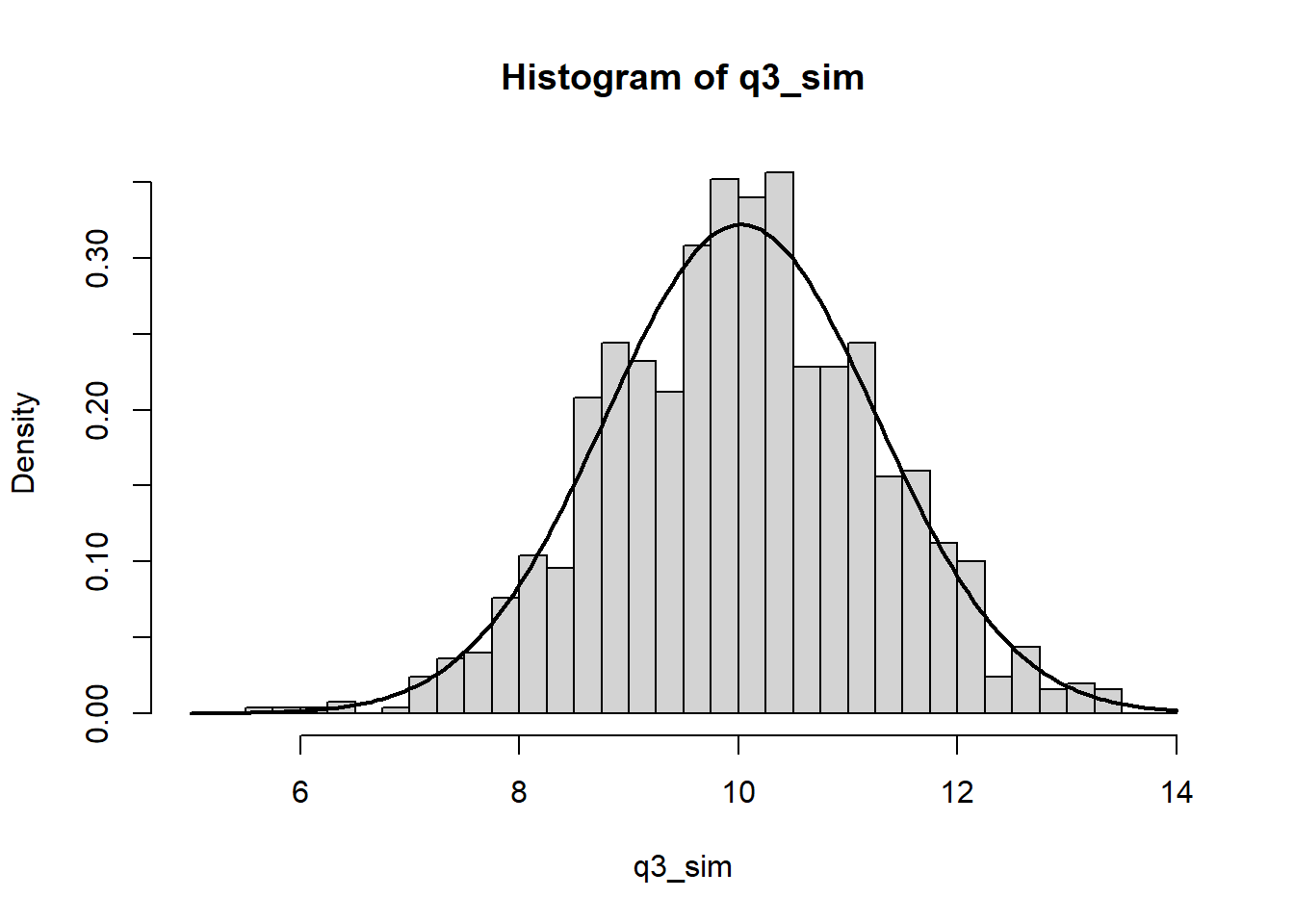
The normal density curve is the normal distribution implied by the observed mean and variance of the simulated data. While the histogram matches the density curve fairly well, there are a few regions close to the mean which are sparser than we would expect – likely because we just haven’t done enough simulations to see the distribution in full detail.
Q4
Distribution of averages and differences: the heights of men in the United States are approximately normally distributed with mean 69.1 inches and standard deviation 2.9 inches. The heights of women are approximately normally distributed with mean 63.7 inches and standard deviation 2.7 inches. Let \(x\) be the average height of 100 randomly sampled men, and \(y\) be the average of 100 randomly sampled women. Create 1000 simulations of \(x-y\) and plot their histogram. Using the simulations, compute the mean and standard deviation of the distribution of \(x-y\) and compare to their exact values.
The exact values of the mean and standard deviation of \(x-y\) are \(5.4\) and \(0.4\) respectively (mentioned earlier in the chapter). We can do the simulation as follows.
set.seed(371)
q4_sim <- replicate(
    1e3,
    mean(rnorm(100, 69.1, 2.9)) - mean(rnorm(100, 63.7, 2.7))
)
q4_mean <- mean(q4_sim)
q4_sd <- sd(q4_sim)
hist(q4_sim, breaks = seq(4, 7, 0.1), freq = FALSE)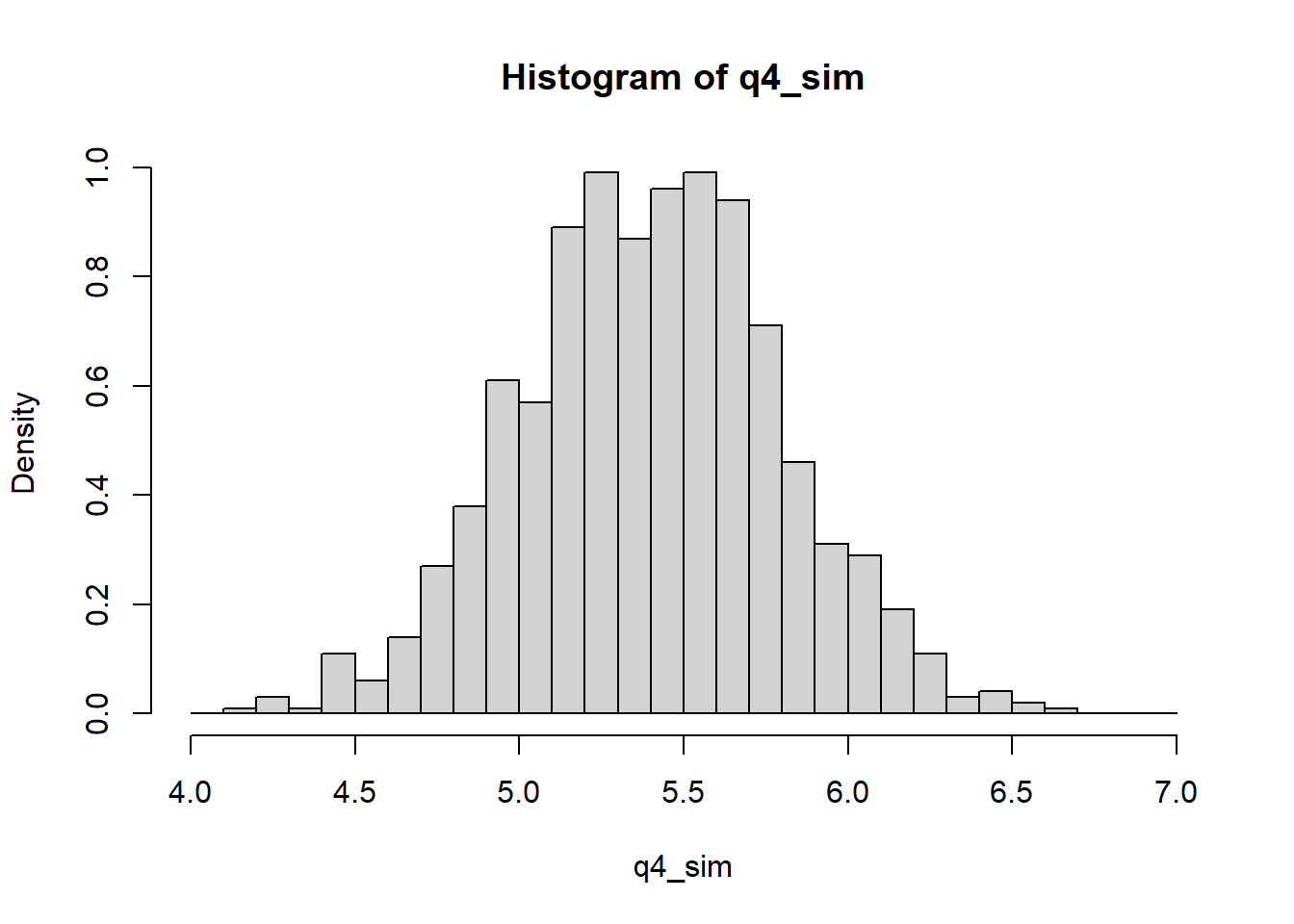
The observed mean from the simulation is \(5.3988\) and the observed SD is \(0.3963\). The simulation results are basically the same as the theoretical values.
Q5
Correlated random variables: suppose that the heights of husbands and wives have a correlation of 0.3. Let \(x\) and \(y\) be the heights of a married couple chosen at random. What are the mean and standard deviation of the average height, \((x + y)/2\)?
Let \(\mu_x\) and \(\sigma_x\) be the mean and standard deviation of \(X\) respectively, and let \(\mu_y\) and \(\sigma_y\) be the mean and standard deviation of \(Y\) respectively. Then, the mean and standard deviation of \(x+y\) are \[ \mu_x + \mu_y \quad \text{and} \quad \sqrt{\sigma^2_x + \sigma^2_y - 2\rho\sigma_x\sigma_y} \] respectively. Now, the mean of \(X/2\) is \(\mu_x/2\) and similar for the mean of \(Y/2\). The standard deviation of \(X/2\) is \(\sigma_x / 2,\) and similar for the standard deviation of \(Y/2\). So then, using the numbers from the previous question text, we get that the mean of \((x+y)/2\) is \[ \frac{1}{2}(\mu_x + \mu_y) = \frac{1}{2}(69.1 + 63.7) = 66.4, \] and the standard deviation is \[ \frac{1}{2}\sqrt{(2.9)^2 + (2.7)^2 + 2(0.3)(2.9)(2.7)} = 2.26. \]
We can also test these theoretical averages against an empirical simulation using the mvtnorm package.
set.seed(372)
mu <- c(69.1, 63.7)
sigma <- matrix(c(2.9 ^ 2, 0.3 * 2.9 * 2.7, 0.3 * 2.9 * 2.7, 2.7 ^ 2), ncol = 2)
sim_q5 <- mvtnorm::rmvnorm(1000, mu, sigma)
sim_avgs <- rowMeans(sim_q5)
mean(sim_avgs)
[1] 66.37027sd(sim_avgs)[1] 2.266538