library(latex2exp)
options("scipen" = 9999, "digits" = 16)
Notes
I actually took notes this time! I already know a pretty good amount about the beta distribution, but I’ve never used it like this before.
- Motivation: an event occurs with an unknown probability. How do we estimate the probability of occurrence? E.g. if you flip a coin 20 times and observe 7 heads, what is the probability of getting heads?
- Black box problem: you put in a quarter. Sometimes the quarter disappears and sometimes it gives you the quarter back. Sometimes it also gives you two quarters. Suppose we try 40 times and we get two quarters 14 times. Then, we could suppose that
\[\begin{align*} H_1 &: P(\text{two quarters}) = \frac{1}{2} \text{ and} \\ H_2 &: P(\text{two quarters}) = \frac{14}{41}. \end{align*}\]
Using a binomial likelihood to calculate the probability of each hypothesis, we would get that \[\begin{align*} P(D \mid H_1) &= \mathcal{B}\left(14 \mid 41, \frac{1}{2}\right) \approx 0.016, \\ P(D \mid H_2) &= \mathcal{B}\left(14 \mid 41, \frac{14}{41}\right) \approx 0.130, \text{ and therefore} \\ \frac{P(D \mid H_2)}{P(D \mid H_1)} &\approx 8.125. \end{align*}\] But even though \(H_2\) appears much more likely, neither is impossible!
- We could also take a systematic sample of potential probabilities over the range \((0, 1)\), since we have observed both outcomes – these would be our “hypotheses”. Plotting this likelihood curve over the possible values of \(p\) would look like this.
p <- seq(0.01, 0.99, 0.01)
plot(
    p, dbinom(14, 41, p), type = "l", lty = 2,
    xlab = TeX('$\\hat{p}$'),
    ylab = TeX('$P(D \\ | \\ \\hat{p})$')
)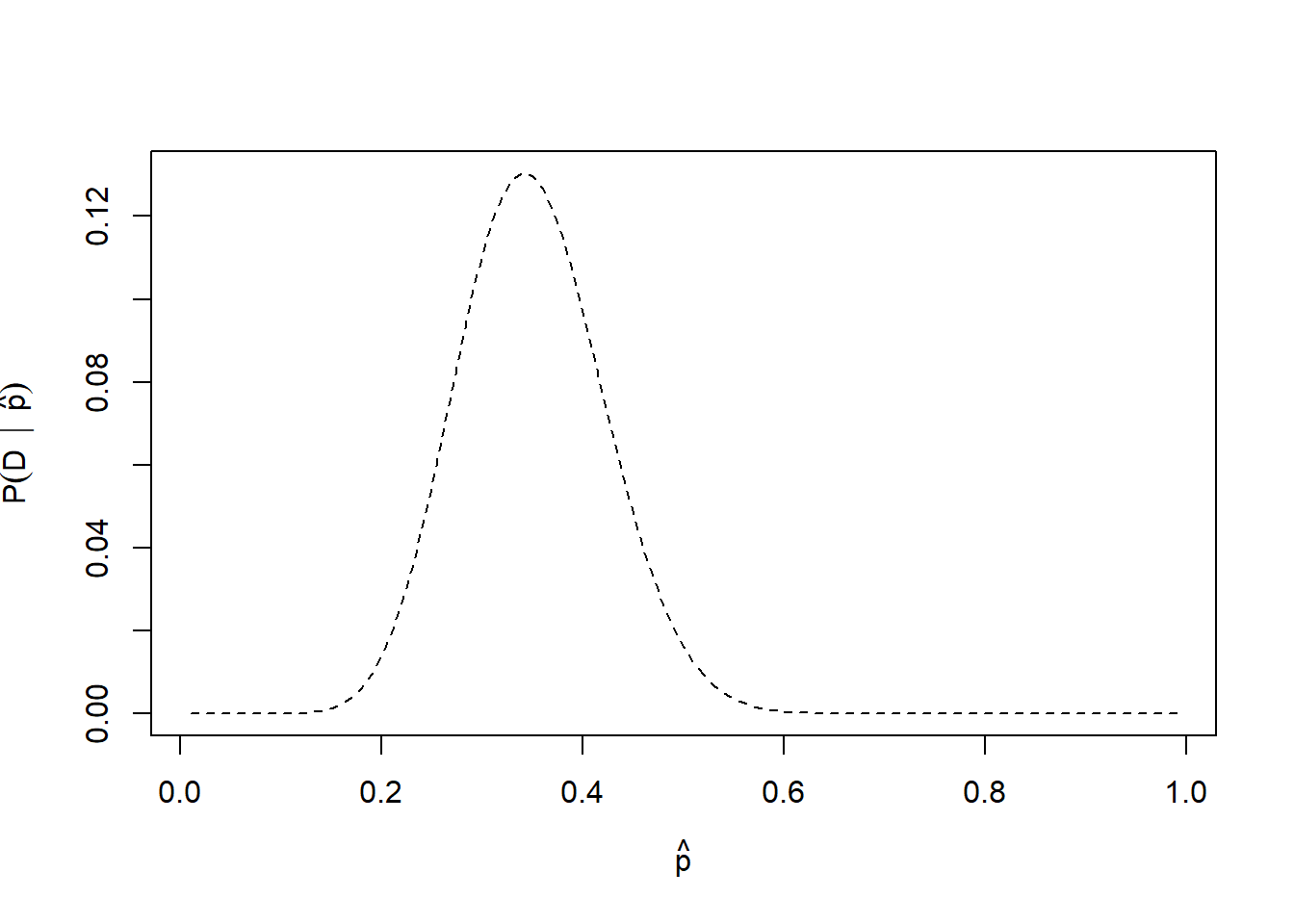
- These discrete values approximate a beta distribution (a fact that we will not prove). The functional form of the Beta distribution is given by
\[\text{Beta}\left( p; \alpha, \beta \right) = \frac{p^{\alpha - 1}(1-p)^{\beta - 1}}{\mathrm{B}(\alpha, \beta)},\] where \(\mathrm{B}(a, b)\) is the beta function, defined as \[\mathrm{B}(a, b) = \int_0^1 t^{a-1}(1-t)^{b-1} \ \mathrm{d}t = \frac{\Gamma(a)\Gamma(b)}{\Gamma(a + b)}.\]
The beta function acts as a normalizing constant in this case.
To use this for getting the same curve, use: + \(p\): the probability of the event; + \(a\): how many times we observe a success; + \(b\): how many times we observe a failure.
- What if we want to know the probability that the true chance of getting back two quarters from the black box is less than \(\frac{1}{2}\)? (As a quick note, the probability that it will be exactly \(\frac{1}{2}\) is zero. With continuous distributions, all single outcomes have zero probability, we can only calculate the probability of ranges.) We can calculate:
\[P\left(p \leq \frac{1}{2}\right) = \int_{0}^{1/2} \ \frac{p^{14-1}(1-p)^{27-1}}{\mathrm{B}(14, 27)} \ \mathrm{d}p.\]
We can get this in R via numerical integration (more details on this in the first exercise).
integrate(function(p) dbeta(p, 14, 27), 0, 0.5)0.9807613458578994 with absolute error < 0.0000059There is a 98% chance, given our evidence, that the probability of getting two coins back is less than one half.
Quick workthrough of the Gacha game example!
- \(n = 1000\) trials
- \(k = 5\) Bradley Efron cards
- We’ll model this with a \(\mathrm{Beta}(5, 1195)\) distribution.
- Our friend will play the game if \(P(p \geq 0.005) > 70\%\).
integrate(function(x) dbeta(x, 5, 1195), 0.005, 1)0.2850559397969717 with absolute error < 0.0001So the probability is only \(29\%\), so our friend will not play the game.
Solutions
Q1
You want to use the beta distribution to determine whether or not a coin you have is a fair coin — meaning that the coin gives you heads and tails equally. You flip the coin 10 times and get 4 heads and 6 tails. Using the beta distribution, what is the probability that the coin will land on heads more than 60 percent of the time?
The probability we are interested in is \[P(p \geq 0.6) = \int_0^{0.6} \mathrm{Beta}(p, 4, 6) \ \mathrm{d}p.\]
We could, of course, write out the distribution and integrate it: \[P(p \geq 0.6) = \int_0^{0.6} \frac{1}{\mathrm{B} \left(4, 6\right)}p^{4-1}(1-p)^{6-1} \ \mathrm{d}p.\]
Here, \(\mathrm{B}(a, b)\) is the beta function, not the binomial distribution. In general, we could integrate \[\int p^{a - 1}(1-p)^{b - 1} \ \mathrm{d}p \] for real, known constants \(k, a, b\), but the general integral in terms of \(a\) and \(b\) is non-elementary, so it is impractical to do this symbolically. The solution to this integral is called the “regularized incomplete beta function”, \(I_x(a, b).\) That means the solution to our original integral is \[ P(p \geq 0.6) = I_{0.6}(4, 6) = \frac{\mathrm{B}_{0.6}(4, 6)}{\mathrm{B}(4, 6)}, \] which we can’t actually calculate in base R (there is no built-in function for the incomplete beta function, although there could be a math identity that I don’t know that lets us calculate it with the tools at our disposal). Apparently this does not come up too often (for reasons we will see shortly), but there are a few packages that offer the incomplete beta function. I found: spsh, UCS, and the one I’ll load, zipfR. These all do other things so it seems potentially worthwhile to me to implement a package that ONLY includes the incomplete beta and gamma functions.
zipfR::Ibeta(0.6, 4, 6) / beta(4, 6)[1] 0.9006474239999999Note that we could get the same thing by numerical integration.
integrate(
    f = \(p) (1 / beta(4, 6)) * p ^ 3 * (1 - p) ^ 5,
    lower = 0,
    upper = 0.6
)
0.9006474239999995 with absolute error < 0.00000000000001The two values are the same to like 15 digits of precision. So we really don’t need to go through all of that mess, we can just use numerical integration. As you may have guessed, R has multiple easier ways to do this. First, the beta density is already built into R, so we don’t have to write out the entire thing.
integrate(
    f = \(p) dbeta(p, 4, 6),
    lower = 0,
    upper = 0.6
)
0.900647424 with absolute error < 0.00000000000001And of course, R has a built-in, better way to get this probability than using the standard numerical integrator. (And since the beta distribution is continuous, we don’t even have to worry about the boundaries this time.)
pbeta(0.6, 4, 6, lower.tail = TRUE)[1] 0.9006474239999999Q2
You flip the coin 10 more times and now have 9 heads and 11 tails total. What is the probability that the coin is fair, using our definition of fair, give or take 5%?
So, we can either numerically integrate, which allows us to specify whatever bounds we want (since this integrand is pretty well-behaved for this kind of thing).
integrate(
    f = \(p) dbeta(p, 9, 11),
    lower = 0.45,
    upper = 0.55
)
0.3098800156513043 with absolute error < 0.0000000000000034Or we can just subtract.
pbeta(0.55, 9, 11) - pbeta(0.45, 9, 11)[1] 0.3098800156513036Sometimes subtraction can be a problem with numerical computing, but if subtraction will cause a problem, so will numerical integration, so this latter method is what I would default to.
Q3
Data is the best way to become more confident in your assertions. You flip the coin 200 more times and end up with 109 heads and 111 tails. Now what is the probability that the coin is fair, give or take 5%?
Alright, I’ve already talked enough about how to solve these problems, this is just another of the same thing. So let’s just solve it.
pbeta(0.55, 109, 111) - pbeta(0.45, 109, 111)[1] 0.8589371426532764That’s a pretty good chance, I think.