Chapter 9: Bayesian Priors and Working with Probability Distributions

options("scipen" = 9999, "digits" = 4)

This chapter introduces the concept of a prior probability distribution, rather than a single point prior (which is also, technically, a prior distribution, but it is the degenerate distribution which is very boring).

Q1

A friend finds a coin on the ground, flips it, and gets six heads in a row and then one tails. Give the beta distribution that describes this. Use integration to determine the probability that the true rate of flipping heads is between 0.4 and 0.6, reflecting the belief that the coin is reasonably fair.

The beta distribution associated with the data we observed is \[\text{Beta}(\alpha = 6, \beta = 1),\] since flipping heads is the outcome of interest (the “success”). Integrating over the specified range, we get that \[P(0.4 \leq p \leq 0.6) = \int_{0.4}^{0.6} \text{Beta}(p \mid 6, 1) \ \mathrm{d}p. \] Approximating the integral in R, we get the following result.

(q1res <- integrate(f = \(x) dbeta(x, 6, 1), lower = 0.4, upper = 0.6))

0.04256 with absolute error < 0.00000000000000047

Our prior probability that the true probability of flipping heads is between 0.4 and 0.6 is approximately \(4.26\%\).

Q2

Come up with a prior probability that the coin is fair. Use a beta distribution such that there is at least a 95% chance that the true rate of flipping heads is between 0.4 and 0.6.

We want to find a prior probability which guarantees \[0.95 \leq \int_{0.4}^{0.6} \text{Beta}(p \mid \alpha, \beta) \ \mathrm{d}p.\]

We know that \(\text{Beta}(1, 1)\) is uniform, so the probability will be too small in the interval we want. If we increase both numbers at the same time so that \(\alpha = \beta\), we know that \(p=0.5\) will be the most likely value, which is desirable for the prior we want to construct. So, if we instead take \(\alpha = 6\) and \(\beta = 6\), we get the following result.

(q2res1 <- integrate(f = \(x) dbeta(x, 6, 6), lower = 0.4, upper = 0.6))

0.507 with absolute error < 0.0000000000000056

We see that this prior still isn’t strong enough to give us the coverage we want in the given range. So let’s try doubling both of the parameters.

(q2res2 <- integrate(f = \(x) dbeta(x, 12, 12), lower = 0.4, upper = 0.6))

0.6727 with absolute error < 0.0000000000000075

Even this still doesn’t work – we need an extremely strong beta prior to guarantee the probability we are interested in. So now I’ll experiment with numbers, testing a grid until we get what we want.

parms <- 1:100
q2res3 <- sapply(
    parms,
    \(ab) integrate(f = \(x) dbeta(x, ab, ab), lower = 0.4, upper = 0.6)$value
)

# Get the minimum number where the probability is above the target.
prior_parm <- parms[[which(q2res3 >= 0.95)[[1]]]]

We can obtain the correct probability bound by using a beta distribution where both parameters are equal to \(48\).

Q3

Now see how many more heads (with no more tails) it would take to convince you that there is a reasonable chance that this coin is not fair. In this case, let’s say that this means that our belief in the rate of the coin being between 0.4 and 0.6 drops below 0.5.

We know that the posterior distribution after we observe \(k\) more heads is equal to \[\text{Beta}(\alpha = 48 + k, \beta = 48),\] so now what we want to find is \[ \operatorname*{arg\,min}_k \int_{0.4}^{0.6} \text{Beta}(p \mid 48 + k, 48) \ \mathrm{d}p. \] We’ll estimate \(k\) using a grid search.

k_vals <- 1L:100L
integral_values <- sapply(
    k_vals,
    \(k) integrate(
        f = \(x) dbeta(x, prior_parm + k, prior_parm),
        lower = 0.4,
        upper = 0.6
    )$value
)
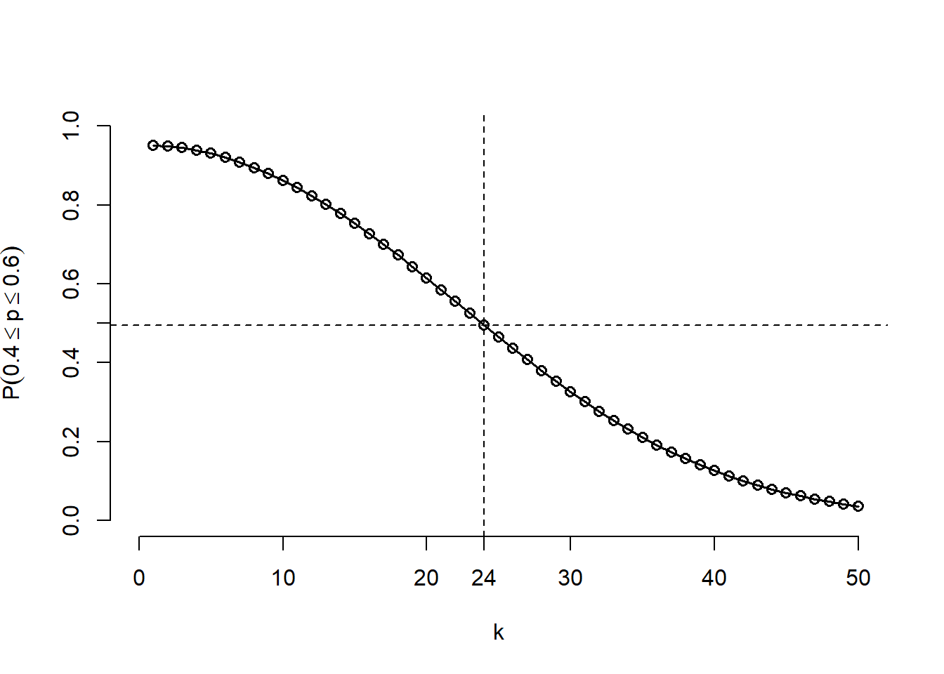
(min_k <- k_vals[which(integral_values < 0.5)[[1]]])

[1] 24

So it would take 24 more heads in a row without any tail flips before our credibility that the coin is unfair is \(50\%\) or higher.

We can make a plot of the results as well to see this.

plot(
    NULL, NULL,
    xlim = c(0, 50), ylim = c(0, 1),
    xlab = latex2exp::TeX(r'($k$)'),
    ylab = latex2exp::TeX(r'($P(0.4 \leq p \leq 0.6)$)'),
    axes = FALSE
)
axis(1, at = c(seq(0, 50, 10), min_k))
axis(2, at = c(seq(0, 1, 0.2), 0.5))
abline(h = integral_values[min_k], lty = 2)
abline(v = min_k, lty = 2)
lines(1:50, integral_values[1:50], type = "o", lwd = 1.5)