Chapter 13: The Tools of Parameter Estimation

options("scipen" = 9999, "digits" = 4)

This chapter covers using the PDF, CDF, and quantiles for distributions.
Notably, the book explains that they use the word “confidence interval” when they are actually talking about Bayesian credible intervals – there is really no reason for them to do this and it is confusing.

Q1

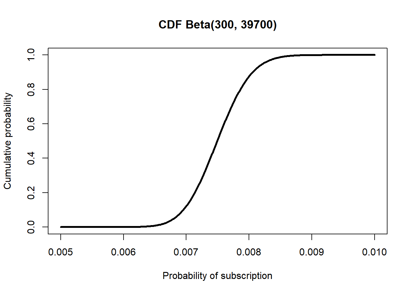
Using the code example for plotting the PDF on page 127, plot the CDF and quantile functions.

xs <- seq(0.005, 0.01, by = 1e-5)
plot(
    xs,
    pbeta(xs, 300, 4e4 - 300),
    type = "l", lwd = 3,
    xlab = "Probability of subscription",
    ylab = "Cumulative probability",
    main = "CDF Beta(300, 39700)"
)

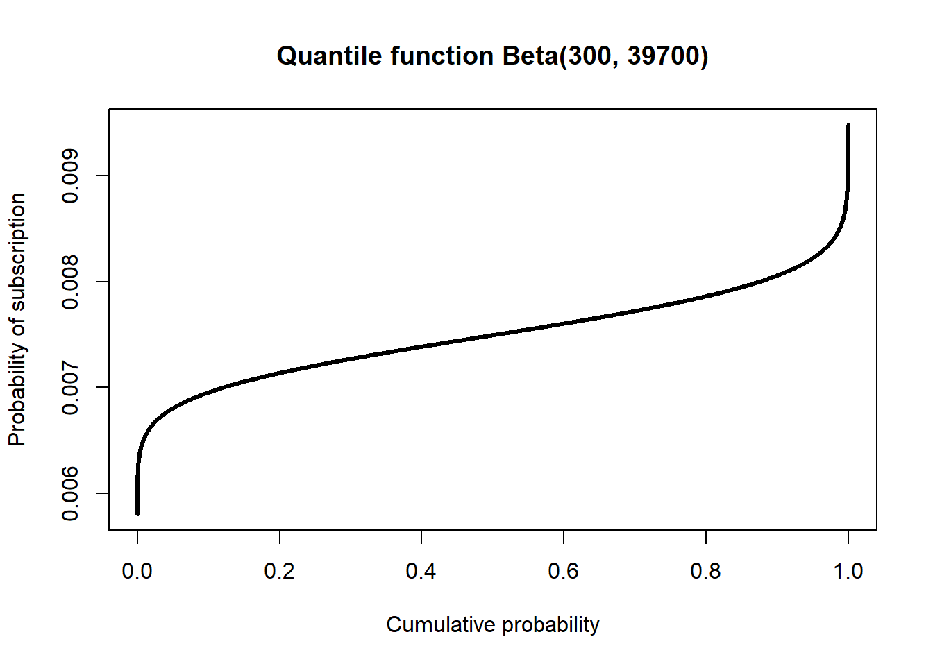
xs <- seq(1e-5, 1 - 1e-5, 1e-5)
plot(
    xs,
    qbeta(xs, 300, 4e4 - 300),
    type = "l", lwd = 3,
    ylab = "Probability of subscription",
    xlab = "Cumulative probability",
    main = "Quantile function Beta(300, 39700)"
)

Q2

Returning to the task of measuring snowfall from Chapter 10, say you have the following measurements (in inches) of snowfall:

7.8, 9.4, 10.0, 7.9, 9.4, 7.0, 7.0, 7.1, 8.9, 7.4.

What is your 99.9% confidence interval for the true value of snowfall?

Assuming the snowfall measurements are normally distributed, first we need to calculate the mean and standard deviation of the measurements.

snow <- c(7.8, 9.4, 10.0, 7.9, 9.4, 7.0, 7.0, 7.1, 8.9, 7.4)
(snow_mean <- mean(snow))

[1] 8.19

(snow_sd <- sd(snow))

[1] 1.135

Now to obtain a \(99.9\%\) credible interval, we need to calculate quantiles where the probabilities are \(0.0005\) and \(0.9995\).

(snow_ci <- qnorm(c(0.0005, 0.9995), snow_mean, snow_sd))

[1]  4.456 11.924

So our estimate for the actual snowfall is 8.19 inches with a \(99.9\%\) credible interval of \((4.46, 11.92)\).

Q3

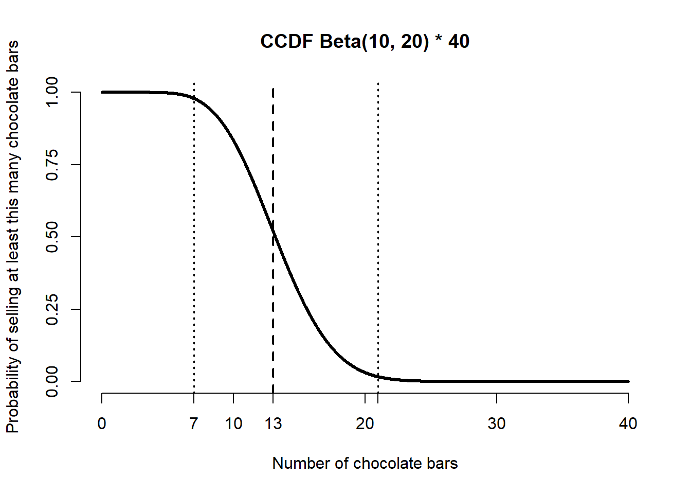
A child is going door to door selling candy bars. So far she has visited 30 houses and sold 10 candy bars. She will visit 40 more houses today. What is the 95% confidence interval for how many candy bars she will sell the rest of the day?

We’ll model the probability, say \(\pi\) that a house will buy chocolate bars using a beta distribution. Based on the information we have so far, we should assume that \[\pi \sim \mathcal{B}(10, 20).\]

We can then calculate the mean and the 95% confidence interval using the distribution.

(mean_pi <- 10 / 30)

[1] 0.3333

(ci_pi <- qbeta(c(0.025, 0.975), 10, 20))

[1] 0.1794 0.5083

So, if she visits 40 more houses today, we can calculate the number of houses we expect to buy chocolate for each of those probability estimates.

(mean_choc <- mean_pi * 40)

[1] 13.33

(ci_choc <- ci_pi * 40)

[1]  7.175 20.333

So we would expect \(13\) houses to buy chocolate if the trend stays the same, with a \(95\%\) credible interval of \((7, 21)\). (Note that the interval is not exact due to rounding, but it is the closest we can get with integer boundaries.)

We can also make a plot of the expected number of chocolate bars.

xs <- seq(1e-5, 1 - 1e-5, 1e-5)
plot(
    NULL, NULL,
    ylab = "Probability of selling at least this many chocolate bars",
    xlab = "Number of chocolate bars",
    main = "CCDF Beta(10, 20) * 40",
    xlim = c(0, 40),
    ylim = c(0, 1),
    axes = FALSE
)

abline(v = floor(mean_choc), lty = 2, lwd = 2)
abline(v = floor(ci_choc[[1]]), lty = 3, lwd = 1.5)
abline(v = ceiling(ci_choc[[2]]), lty = 3, lwd = 1.5)
lines(
    xs * 40,
    1 - pbeta(xs, 10, 20),
    type = "l", lwd = 3
)
axis(
    1,
    at = c(seq(0, 40, 10), floor(mean_choc), floor(ci_choc[[1]]),
                 ceiling(ci_choc[[2]]))
)
axis(2, at = seq(0, 1, 0.25))