options("scipen" = 9999, "digits" = 4)Q1
Suppose you’re playing air hockey with some friends and flip a coin to see who starts with the puck. After playing 12 times, you realize that the friend who brings the coin almost always seems to go first: 9 out of 12 times. Some of your other friends start to get suspicious. Define prior probability distributions for the following beliefs:
- One person who weakly believes that the friend is cheating and the true rate of coming up heads is closer to 70 percent.
- One person who very strongly trusts that the coin is fair and provided a 50 percent chance of coming up heads.
- One person who strongly believes the coin is biased to come up heads 70 percent of the time.
We’ll use a beta distribution for all three of the priors. For the first prior, we want a beta distribution with a mean that’s close to 70 percent, but we want the variance to be fairly high. The easiest way to do this, is to use \(\alpha = 7\) and \(\beta = 3\), which we know will have a mean of exactly \(70\%\) but will still be fairly spread out.
For the second prior, we’ll use a beta distribution with equal parameters. Since their belief is fairly strong, we’ll say \(\alpha = 10\), \(\beta = 10\). Finally, for the third person, we’ll use \(\alpha = 700\), \(\beta = 300\), which will have a mean of \(70\%\) but with little variation.
Let’s plot the three priors. The code for this plot is somewhat long, so it has been hidden by default.
Code
# Setup
pal <- gray.colors(3, start = 0, end = 0.75)
xs <- seq(1e-5, 1 - 1e-5, length.out = 1000)
layout(matrix(c(1, 2), nrow = 1))

# PDF plot
p1 <- dbeta(xs, 7, 3)
p2 <- dbeta(xs, 10, 10)
p3 <- dbeta(xs, 700, 300)
plot(
    NULL, NULL,
    xlab = "Probability of the coin being heads",
    ylab = "Prior density (truncated at 4)",
    xlim = c(0, 1), ylim = c(0, 4),
    axes = FALSE,
    main = "Friends' prior PDFs"
)
lines(xs, p1, lwd = 3, col = pal[[1]], lty = 1)
lines(xs, p2, lwd = 3, col = pal[[2]], lty = 2)
lines(xs, p3, lwd = 3, col = pal[[3]], lty = 3)
axis(1, seq(0, 1, 0.25))
axis(2, seq(0, 4, 1))
legend(
    x = 0, y = 3.9,
    legend = c("Friend 1", "Friend 2", "Friend 3"),
    col = pal,
    lty = 1:3,
    lwd = 3
)

# CDF plot
c1 <- pbeta(xs, 7, 3)
c2 <- pbeta(xs, 10, 10)
c3 <- pbeta(xs, 700, 300)
plot(
    NULL, NULL,
    xlab = "Probability of the coin being heads",
    ylab = "Cumulative prior probability",
    xlim = c(0, 1), ylim = c(0, 1),
    axes = FALSE,
    main = "Friends' prior CDFs"
)
lines(xs, c1, lwd = 3, col = pal[[1]], lty = 1)
lines(xs, c2, lwd = 3, col = pal[[2]], lty = 2)
lines(xs, c3, lwd = 3, col = pal[[3]], lty = 3)
axis(1, seq(0, 1, 0.25))
axis(2, seq(0, 1, 0.25))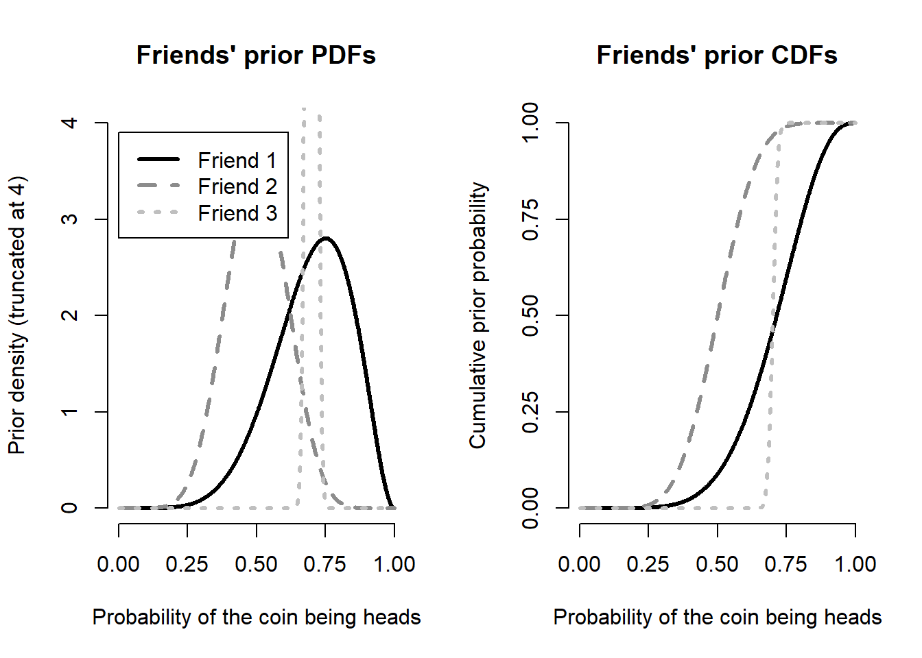
We can see that friend 3 is so certain, the PDF plot had to be truncated in order to see the other two curves.
To test the coin, you flip it 20 more times and get 9 heads and 11 tails. Using the priors you calculated in the previous question, what are the updated posterior beliefs in the true rate of flipping a heads in terms of the 95 percent confidence interval?
OK. now we need to compute the posteriors for each of the three friends.
post1 <- dbeta(xs,  7 + 9,  3 + 11)
post2 <- dbeta(xs, 10 + 9, 10 + 11)
post3 <- dbeta(xs, 70 + 9, 30 + 11)
Next we need to calculate the posterior credible intervals.
ci_levels <- c(0.025, 0.975)
post_cis <-
    rbind(
        qbeta(ci_levels, 07 + 9, 03 + 11),
        qbeta(ci_levels, 10 + 9, 10 + 11),
        qbeta(ci_levels, 70 + 9, 30 + 11)
    ) |>
    `colnames<-`(c("lower", "upper")) |>
    tibble::as_tibble() |>
    tibble::add_column(friend = paste(1:3))
print(post_cis)
# A tibble: 3 × 3
lower upper friend
<dbl> <dbl> <chr>
1 0.357 0.706 1
2 0.324 0.628 2
3 0.572 0.740 3 Finally, we can visualize the prior and posterior density with the CrI for each of our friends.
Code
# Setup
pal2 <- gray.colors(2, start = 0, end = 0.5)
xs <- seq(1e-5, 1 - 1e-5, length.out = 1000)
layout(matrix(c(1, 2, 3), nrow = 1))

# posterior/prior plots
# Friend 1
plot(
    NULL, NULL,
    main = "Friend 1",
    xlim = c(0, 1), ylim = c(0, 10),
    xlab = "Probability of the coin being heads",
    ylab = "Density",
)
lines(xs, p1,    lwd = 3, col = pal2[[2]], lty = 3)
lines(xs, post1, lwd = 3, col = pal2[[1]], lty = 1)
abline(v = post_cis[[1, 1]], lty = 2, lwd = 1, col = "firebrick2")
abline(v = post_cis[[1, 2]], lty = 2, lwd = 1, col = "firebrick2")

legend(
    x = 0.02, y = 9.75,
    legend = c("Prior", "Posterior", "95% CrI"),
    col = c(rev(pal2), "firebrick2"),
    lty = c(3, 1, 2),
    lwd = c(3, 3, 1)
)

# Friend 2
plot(
    NULL, NULL,
    main = "Friend 2",
    xlim = c(0, 1), ylim = c(0, 10),
    xlab = "Probability of the coin being heads",
    ylab = "Density",
)
lines(xs, p2,    lwd = 3, col = pal2[[2]], lty = 3)
lines(xs, post2, lwd = 3, col = pal2[[1]], lty = 1)
abline(v = post_cis[[2, 1]], lty = 2, lwd = 1, col = "firebrick2")
abline(v = post_cis[[2, 2]], lty = 2, lwd = 1, col = "firebrick2")

# Friend 3
plot(
    NULL, NULL,
    main = "Friend 3",
    xlim = c(0, 1), ylim = c(0, 10),
    xlab = "Probability of the coin being heads",
    ylab = "Density",
)
lines(xs, p3,    lwd = 3, col = pal2[[2]], lty = 3)
lines(xs, post3, lwd = 3, col = pal2[[1]], lty = 1)
abline(v = post_cis[[3, 1]], lty = 2, lwd = 1, col = "firebrick2")
abline(v = post_cis[[3, 2]], lty = 2, lwd = 1, col = "firebrick2")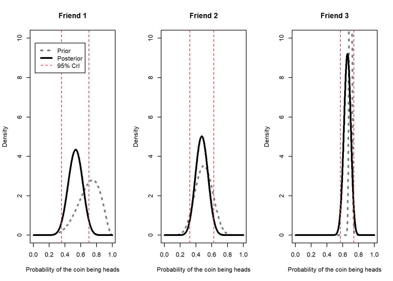
Overall, we can see the following conclusions for each friend:
- Friend 1 did think the coin was unfair before, but is now much more willing to believe the coin is fair given the observed data;
- Friend 2 thought the coin was fair before and is now more confident that the coin is fair given the observed data; and
- Friend 3 still strongly believes the coin is unfair, but the observed data is beginning to change their mind – they are at least now willing to entertain the possibility that the coin is fair.