options("scipen" = 9999, "digits" = 4)Q1
Suppose a director of marketing with many years of experience tells you he believes very strongly that the variant without images (B) won’t perform any differently than the original variant. How could you account for this in our model? Implement this change and see how your final conclusions change as well.
We can account for the director of marketing’s experience by adjusting our priors. To make our prior belief that the conversion rates are the same more stringent, we could use, say, a \(\text{Beta}(300, 700)\) prior.
That means the posterior distribution for variant A is \(\text{Beta}(336, 814)\) and the posterior distribution for variant B is \(\text{Beta}(350, 800)\). We can repeat the Monte Carlo simulation for these priors and draw \(100,000\) samples for each variant.
Code
set.seed(370)
n_sims <- 1e5
a_sims <- rbeta(n_sims, 336, 814)
b_sims <- rbeta(n_sims, 350, 800)

a_density <- density(a_sims, kernel = "epanechnikov")
b_density <- density(b_sims, kernel = "epanechnikov")

plot(
    NULL, NULL,
    xlim = c(0.1, 0.5),
    ylim = c(0, 30),
    xlab = "Conversion rate",
    ylab = "Density",
    main = "Simulated conversion rate distributions for variants A and B",
    axes = FALSE
)
lines(a_density, lwd = 3, col = "dodgerblue2")
lines(b_density, lwd = 3, col = "springgreen3")
axis(1, seq(0.1, 0.5, 0.1))
axis(2, seq(0, 30, 10))
legend(
    0.1, 30, c("A", "B"), col = c("dodgerblue2", "springgreen3"),
    lty = 1, lwd = 3, box.lwd = 0, cex = 1.5
)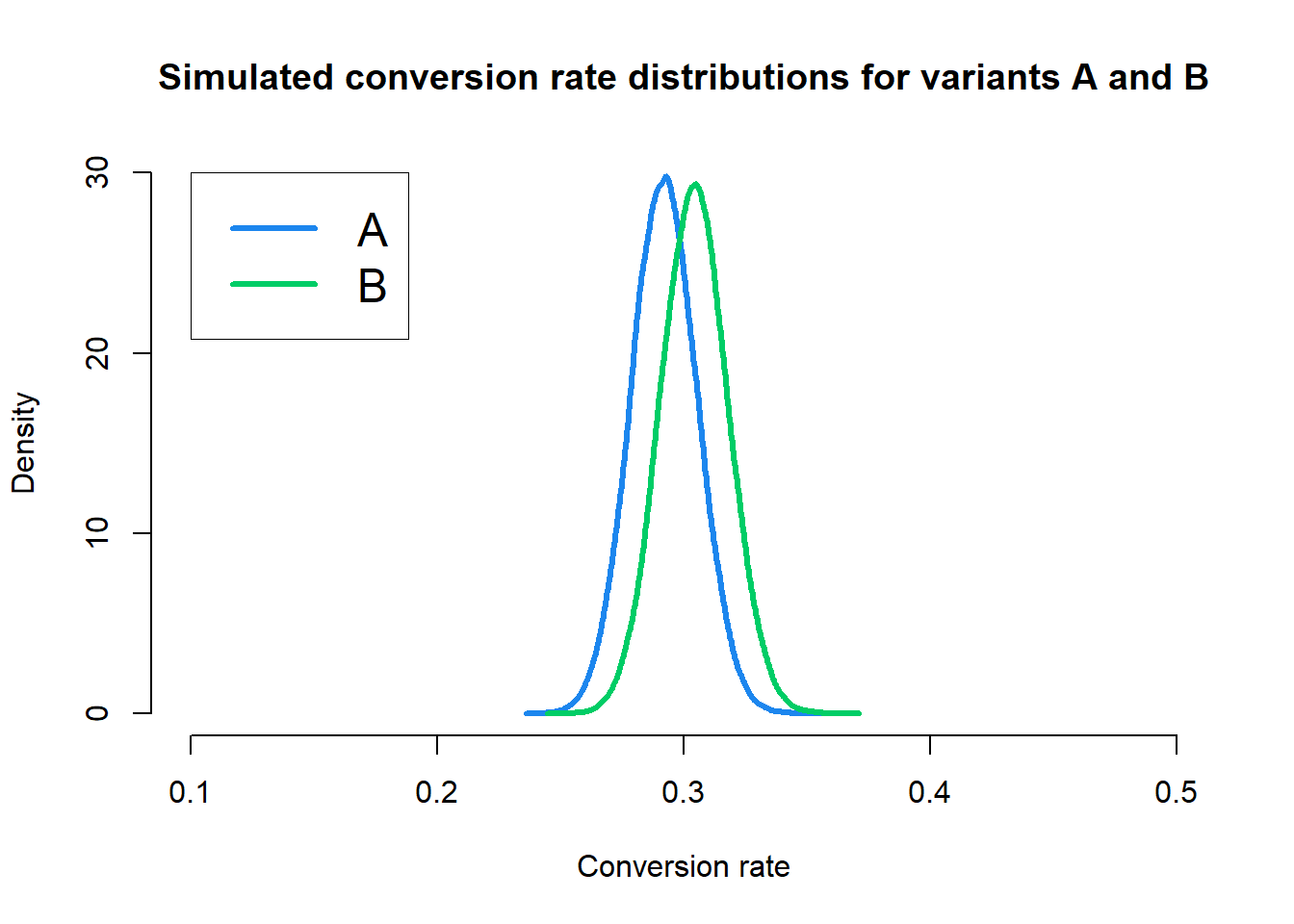
We can see that the posterior distributions for variants A and B are much closer together. In total, \(73.81\%\) of the simulated conversation rates for variant B were greater than the simulated conversation rate for variant A. The empirical CDF for relative improvements is shown below.
Code
imp <- b_sims / a_sims
imp_ecdf <- ecdf(imp)
xs <- seq(min(imp), max(imp), length.out = 1e3)
ys <- imp_ecdf(xs)
plot(
    NULL, NULL,
    main = "Emperical cdf of simulated relative improvements of B over A",
    xlab = "Relative improvement of B over A",
    ylab = "Empirical cumulative probability",
    axes = FALSE,
    xlim = c(0.68, 1.42),
    ylim = c(-0.02, 1.02),
    xaxs = "i", yaxs = "i"
)
abline(h = 0.25, lty = 2, col = "gray")
abline(h = 0.50, lty = 2, col = "gray")
abline(h = 0.75, lty = 2, col = "gray")
abline(v = xs[which.min(abs(ys - 0.25))], lty = 2, col = "gray")
abline(v = xs[which.min(abs(ys - 0.50))], lty = 2, col = "gray")
abline(v = xs[which.min(abs(ys - 0.75))], lty = 2, col = "gray")
lines(
    xs, ys,
    lwd = 3, col = "firebrick4", type = "s",
)
axis(1, seq(0.7, 1.4, 0.1))
axis(2, seq(0, 1, 0.25))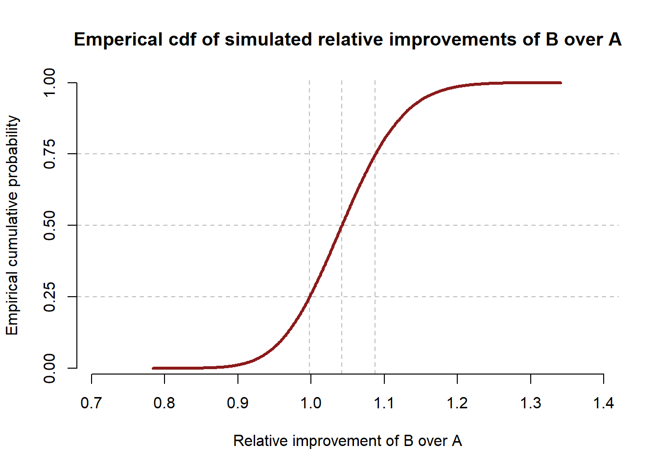
Under the new more stringent prior, we can see that nearly a quarter of all samples showed a higher conversion rate for variant A than variant B, and very few samples showed a relative improvement of variant B more than 1.2. So while our simulation suggests that B is most likely better than A, we are less confident in that assertion, and the magnitude of improvement is estimated to be smaller on average.
Q2
The lead designer sees your results and insists there’s no way that variant B should perform better with no images. She feels that you should assume the conversion rate for variant B is closer to \(20\%\) than \(30\%\). Implement a solution for this and again review the results of our analysis.
To accomodate the lead designer’s prior beliefs, we’ll return to our original prior of \(\text{Beta}(3, 7)\). However, we’ll only use this prior for variant A. For variant B, we want a prior that has a mean conversion rate closer to \(20\%\), so we’ll use \(\text{Beta}(2, 8)\). Let’s take a look at the priors.
Code
xs <- seq(1e-4, 1 - 1e-4, 1e-4)
a_prior_q2 <- dbeta(xs, 3, 7)
b_prior_q2 <- dbeta(xs, 2, 8)

plot(
    NULL, NULL,
    xlim = c(0, 1),
    ylim = c(0, 3.6),
    xlab = "Conversion rate",
    ylab = "Density",
    main = "Prior conversion rate distributions for variants A and B",
    axes = FALSE
)
lines(xs, a_prior_q2, lwd = 3, col = "dodgerblue2")
lines(xs, b_prior_q2, lwd = 3, col = "springgreen3")
axis(1, seq(0, 1, 0.25))
axis(2, seq(0, 3.6, 0.5))
legend(
    0.6, 3.2, c("A", "B"), col = c("dodgerblue2", "springgreen3"),
    lty = 1, lwd = 3, box.lwd = 0, cex = 1.5
)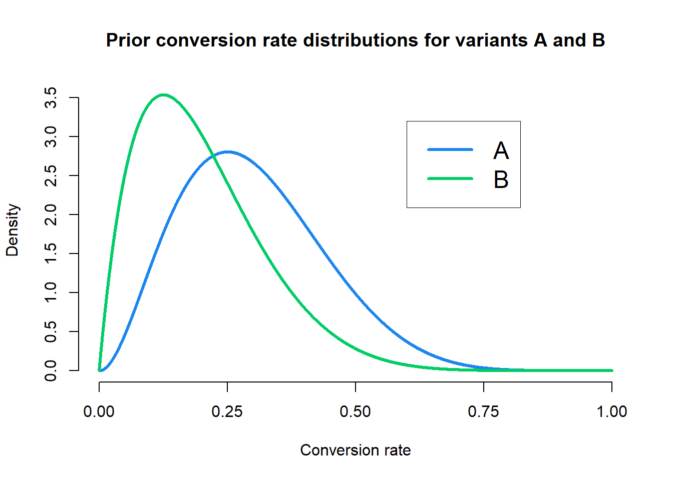
We can see that our priors now assume the average conversion rate for variant B is around \(20\%\) as desired, although both priors are not too strict. So now our posterior distributions given the observed data are \(\text{Beta}(39, 121)\) for variant A and \(\text{Beta}(52, 108)\) for variant B. Let’s take a look at the posterior distributions.
Code
xs <- seq(1e-4, 1 - 1e-4, 1e-4)
a_post_q2 <- dbeta(xs, 39, 121)
b_post_q2 <- dbeta(xs, 52, 108)

plot(
    NULL, NULL,
    xlim = c(0, 1),
    ylim = c(0, 12),
    xlab = "Conversion rate",
    ylab = "Density",
    main = "Posterior conversion rate distributions for variants A and B",
    axes = FALSE
)
lines(xs, a_post_q2, lwd = 3, col = "dodgerblue2")
lines(xs, b_post_q2, lwd = 3, col = "springgreen3")
axis(1, seq(0, 1, 0.25))
axis(2, seq(0, 12, 2))
legend(
    0.6, 10, c("A", "B"), col = c("dodgerblue2", "springgreen3"),
    lty = 1, lwd = 3, box.lwd = 0, cex = 1.5
)
Our posterior distributions again seem to show that the conversion rate for B is, on average, higher than the conversion rate for A. However, the spread of the two posterior distributions is now different and we are less certain in the magnitude of the conversion rate for B than we are for B. Let’s repeat the Monte Carlo simulation with these new priors and look at the ECDF of improvements.
Code
a_sims_q2 <- rbeta(n_sims, 39, 121)
b_sims_q2 <- rbeta(n_sims, 52, 108)
imp_q2 <- b_sims_q2 / a_sims_q2
imp_ecdf_q2 <- ecdf(imp_q2)
xs <- seq(min(imp_q2), max(imp_q2), length.out = 1e3)
ys <- imp_ecdf(xs)
plot(
    NULL, NULL,
    main = "Emperical cdf of simulated relative improvements of B over A",
    xlab = "Relative improvement of B over A",
    ylab = "Empirical cumulative probability",
    axes = FALSE,
    xlim = c(0.48, 3),
    ylim = c(-0.02, 1.02),
    xaxs = "i", yaxs = "i"
)
abline(h = 0.25, lty = 2, col = "gray")
abline(h = 0.50, lty = 2, col = "gray")
abline(h = 0.75, lty = 2, col = "gray")
abline(v = xs[which.min(abs(ys - 0.25))], lty = 2, col = "gray")
abline(v = xs[which.min(abs(ys - 0.50))], lty = 2, col = "gray")
abline(v = xs[which.min(abs(ys - 0.75))], lty = 2, col = "gray")
lines(
    xs, ys,
    lwd = 3, col = "firebrick4", type = "s",
)
axis(1, seq(0.5, 3, 0.5))
axis(2, seq(0, 1, 0.25))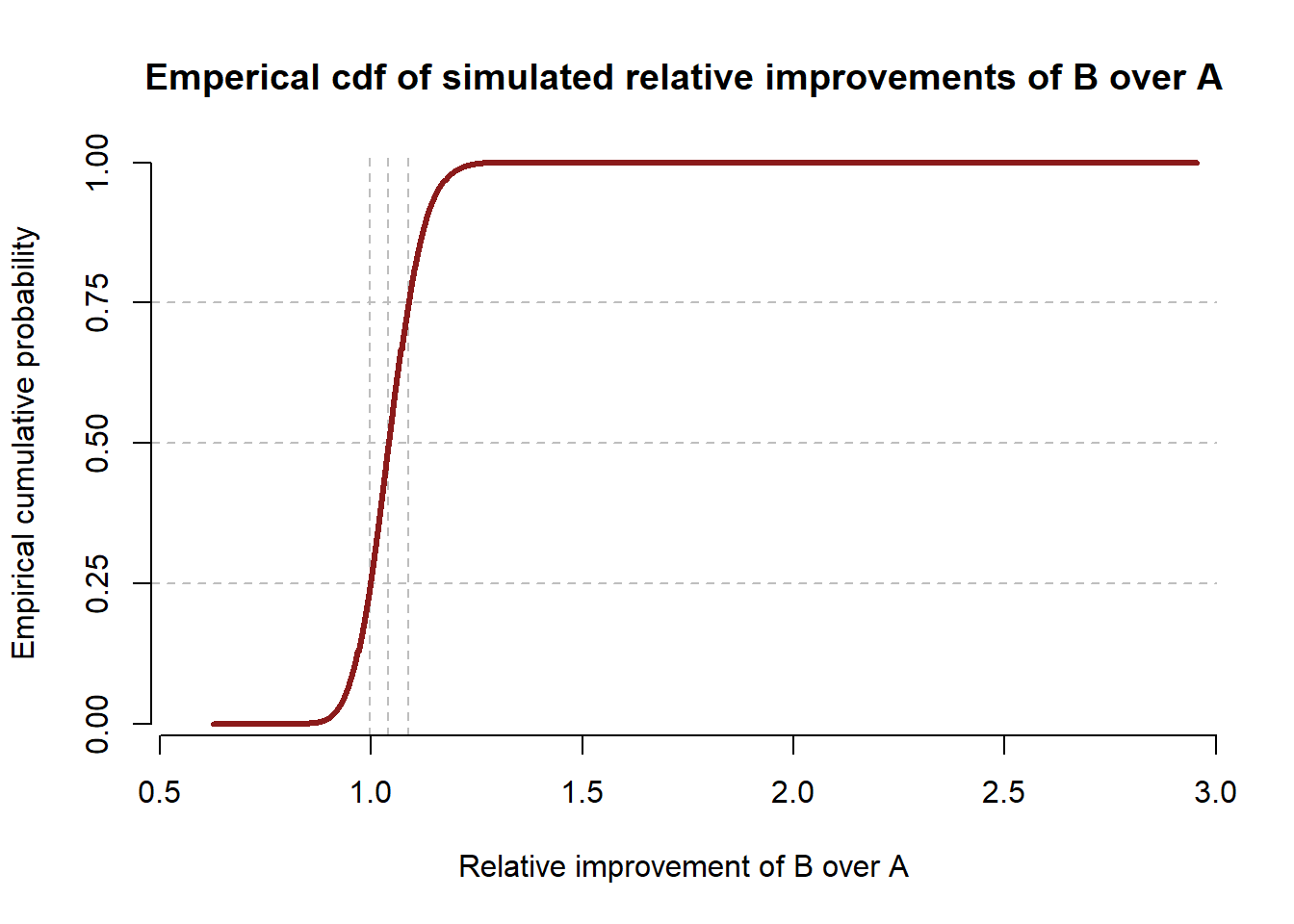
Under these priors, \(94.78\%\) of sampled conversation rates for variant B were higher than the sampled conversion rates for variant A. So despite the lowered probability for variant B, we are still very confident that B outperforms A, although we are slightly less confident than the example in the book using the same priors for B and A.
Q3
Assume that being 95% certain means that you’re more or less “convinced” of a hypothesis. Also assume that there’s no longer any limit to the number of emails you can send in your test. If the true conversion rate for A is 0.25 and the true conversion rate for B is 0.3, explore how many samples it would take to convince the director of marketing that B was in fact superior. Explore the same for the lead designer.
I think this question, like many others in this book, is quite poorly worded. But I’ll assume that what we actually want to know is how many samples we would need to convince either person that the \(P(B > A) = 0.95\).
So, for a number of different sample sizes, we’ll simulate conversions. Then, from those simulated conversion trials (pretend they are real data), we’ll run our original Monte Carlo simulation using the updated prior based on the number of conversion events we observed for variants A and B. We’ll repeat this entire scheme 100 times for both the director and the lead designer in order to make sure our results aren’t due to variance. Then we can plot the results.
Code
# This function runs a single round of our simulation procedure. That is,
# we generate n_samples number of trials, where a trial is defined as one
# variant A email being sent and one variant B email being sent. We simulate
# from the true conversion rate whether those are conversions, and then create
# the posterior and repeat our MC simulation as before.
simulate_probability <- function (
        n_samples, true_a, true_b,
        prior_alpha_a, prior_alpha_b,
        prior_beta_a, prior_beta_b
    ) {
        # Generate the number of conversions in this simulation
        events_a <- runif(n_samples) <= true_a
        events_b <- runif(n_samples) <= true_b

        # Calculate the parameters for the posterior distributions
            post_alpha_a <- prior_alpha_a + sum(events_a)
        post_beta_a <- prior_beta_a + sum(!events_a)
        post_alpha_b <- prior_alpha_b + sum(events_b)
        post_beta_b <- prior_beta_b + sum(!events_b)

        # Now run the Monte Carlo simulation from the implied posterior
        samples_a <- rbeta(1e5, post_alpha_a, post_beta_a)
        samples_b <- rbeta(1e5, post_alpha_b, post_beta_b)

        # Get the probability b > a
        prob_bga <- mean(samples_b > samples_a)
        return(prob_bga)
    }

# This function runs the simulate_probability() function multiple times, each
# time using a different number of samples defined by the samples_seq argument.
# The result is given as a matrix where each column is the output of one
# run of simulate_probability().
run_sample_seq <- function(
        samples_seq = seq(25, 1000, 25),
        ...
    ) {
    sapply(
        samples_seq,
        \(n) simulate_probability(n, ...)
    )
}

# This function will take in our results and return a data frame.
summarize_replicate_results <- function(res, alpha = 0.1) {
    res_mean <- rowMeans(res)
    res_PI <- apply(res, 1, quantile, probs = c(alpha / 2, 1 - alpha / 2))
    out <- data.frame(
        est = res_mean,
        lwr = res_PI[1, ],
        upr = res_PI[2, ]
    )
    return(out)
}

samples_vector <- seq(25, 1000, 25)

# Run the simulation for the director
sims_director <- replicate(
    100,
    run_sample_seq(
        samples_seq = samples_vector,
        true_a = 0.25,
        true_b = 0.35,
        prior_alpha_a = 300,
        prior_alpha_b = 300,
        prior_beta_a = 700,
        prior_beta_b = 700
    )
)
res_director <- cbind(
    n = samples_vector,
    person = 1,
    summarize_replicate_results(sims_director)
)

# And for the designer
sims_designer <- replicate(
    100,
    run_sample_seq(
        samples_seq = samples_vector,
        true_a = 0.25,
        true_b = 0.35,
        prior_alpha_a = 3,
        prior_alpha_b = 7,
        prior_beta_a = 2,
        prior_beta_b = 8
    )
)
res_designer <- cbind(
    n = samples_vector,
    person = 2,
    summarize_replicate_results(sims_designer)
)

# Data cleaning
res_combined <- rbind(res_director, res_designer)
res_combined$person <- factor(
    res_combined$person,
    levels = c(1, 2),
    labels = c("Director of Marketing", "Lead Designer")
)

# Get the intercepts for the number of samples closest to 95% probability
director_n <- res_director$n[which.min(abs(res_director$est - 0.95))]
designer_n <- res_director$n[which.min(abs(res_designer$est - 0.95))]

# Plot the results
library(ggplot2)
res_combined |>
    ggplot() +
    aes(
        x = n, y = est, ymin = lwr, ymax = upr, group = person,
        color = person, fill = person, shape = person
    ) +
    geom_ribbon(alpha = 0.3, color = "transparent") +
    geom_hline(yintercept = 0.95, linetype = 2, linewidth = 1) +
    geom_vline(
        xintercept = c(director_n, designer_n),
        linetype = 2, linewidth = 1
    ) +
    geom_line(linewidth = 1.5, alpha = 0.8) +
    geom_point(size = 3, stroke = 2, fill = "white", alpha = 0.8) +
    scale_color_manual(values = c("dodgerblue2", "firebrick3")) +
    scale_fill_manual(values = c("dodgerblue2", "firebrick3")) +
    scale_shape_manual(values = c(21, 22)) +
    hgp::theme_ms() +
    labs(
        x = "Number of samples",
        y = "Probability of B > A",
        color = NULL,
        fill = NULL,
        shape = NULL
    )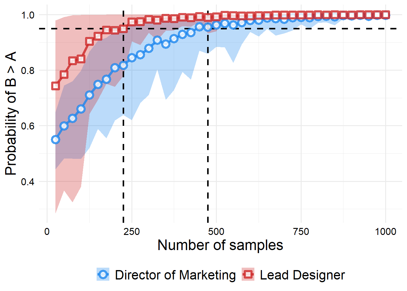
From the plot, we can see that we would need about 250 samples to convince the lead designer, and around 475 samples to convince the director of marketing. However, if we wanted to make sure we take the sampling variability into account, (instead assuming that our lower bound for the probability over all of our sampling replications is 95% or higher), we would actually need around 475 samples to convince the lead designer and 750 samples to convince the director of marketing.