Chapter 19: From Hypothesis Testing to Parameter Estimation

options("scipen" = 9999, "digits" = 4)

Q1

Our Bayes factor assumed that we were looking at \(H_1: P(\text{prize} = 0.5)\). THis allowed us to derive a version of the beta distribution with an alpha of 1 and a beta of 1. Would it matter if we chose a different probability for \(H_1\)? Assume \(H_1: P(\text{prize} = 0.24)\), then see if the resulting distribution, once normalized to sum to 1, is any different from the original hypothesis.

OK, so what we need to do is calculate the new distribution and the old distribution so we can compare them.

hypotheses <- seq(0, 1, by = 0.01)
numerator <- hypotheses ^ 24 * (1 - hypotheses) ^ 76
bf_0.50 <- numerator / (0.50 ^ 24 * (1 - 0.50) ^ 76)
bf_0.24 <- numerator / (0.24 ^ 24 * (1 - 0.24) ^ 76)

# Now normalize the distributions
bf_0.50_norm <- bf_0.50 / sum(bf_0.50)
bf_0.24_norm <- bf_0.24 / sum(bf_0.24)

plot(
    bf_0.24_norm, bf_0.50_norm,
    xlab = "Normalized Bayes factors when assumed probability = 0.24",
    ylab = "Normalized Bayes factors when assumed probability = 0.50",
    pch = 3, cex = 1.1
)
abline(a = 0, b = 1, lty = 2, col = "gray")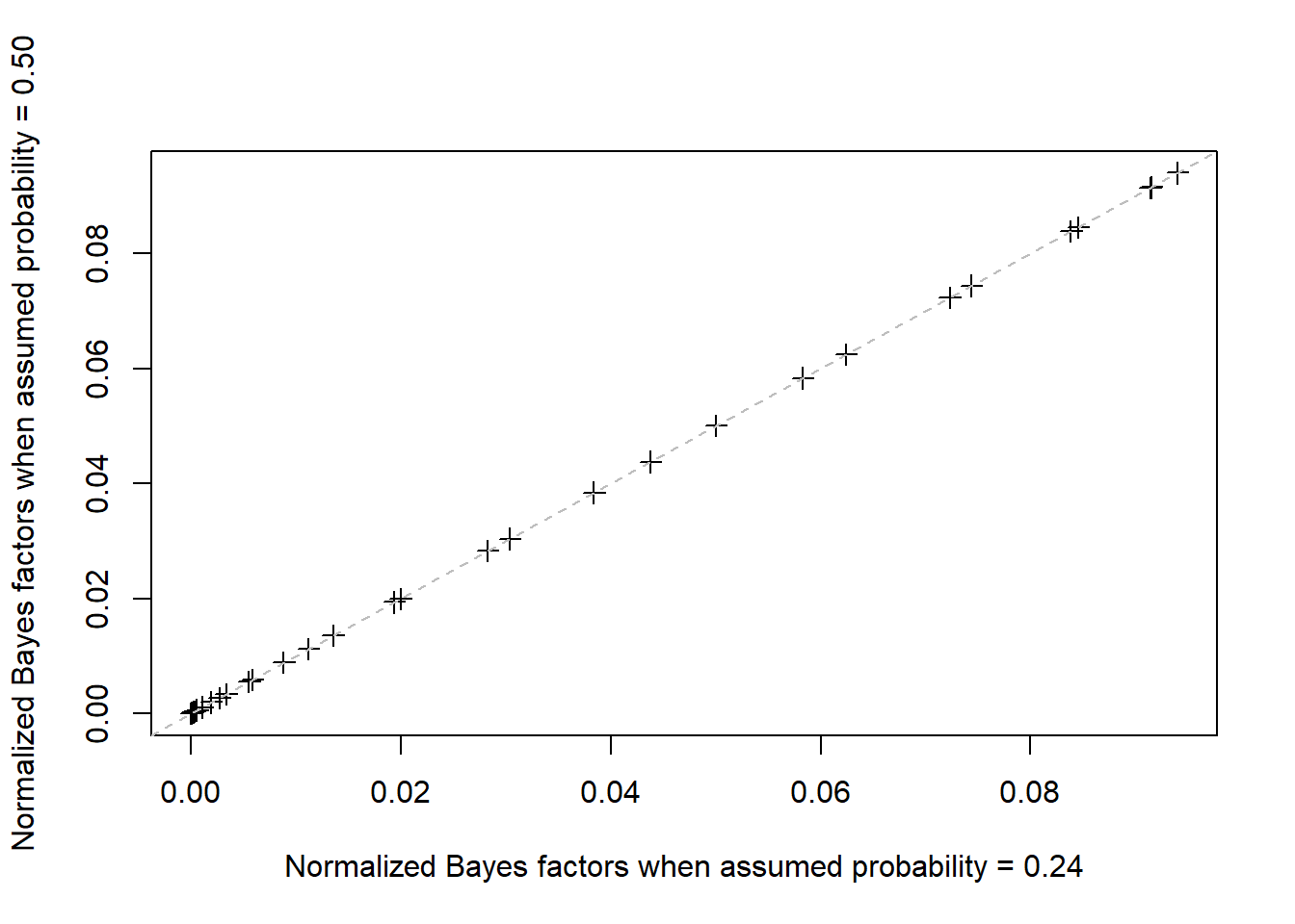

You can see that the points are exactly correlated, i.e., the normalized distributions are exactly the same.

Q2

Write a prior for the distribution in which each hypothesis is 1.05 times more likely than the previous hypothesis (assume our dx remains the same).

First we’ll create the prior.

n <- length(hypotheses)
prior <- 1.05 ^ (0:(n-1))

To obtain the posterior distribution, we multiply the priors by their corresponding Bayes factors and normalize.

post_raw <- prior * bf_0.50_norm
post <- post_raw / sum(post_raw)
plot(
    hypotheses, post, lwd = 3, type = "l",
    xlab = "Hypothesized prize probability",
    ylab = "Normalized posterior density of result"
)

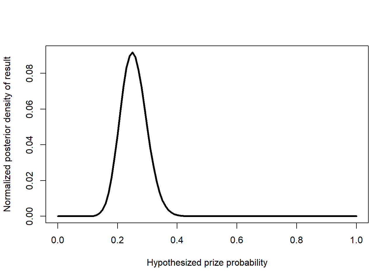
We can see that the best estimate is still around \(0.24\). Even though the extreme values have higher prior likelihood, the evidence is strong enough to ignore them.

Q3

Suppose you observed another duck game that included 34 ducks with prizes and 66 ducks without prizes. How would you set up a test to answer “What is the probability that you have a better chance of winning a prize in this game than in the game we used in our example?”

If we assume a \(\text{Beta}(1, 1)\) prior for both probabilities, then the posterior distribution for the probability of a prize in the first game is \(\text{Beta}(25, 77)\) and the posterior distribution for the probability of a prize in the second game is \(\text{Beta}(35, 67)\). We can conduct a Monte Carlo simulation with, say, \(100,000\) draws from both distributions as we did previously.

set.seed(132)
n_sims <- 1e5
game_1_sim <- rbeta(n_sims, 25, 77)
game_2_sim <- rbeta(n_sims, 35, 67)
prob <- mean(game_2_sim > game_1_sim)

From this simple simulation, the probability that we have a better chance of winning a prize was about \(93.9\%\).

Apparently the solutions in the book wanted us to use arbitrary priors and use a numerical algorithm to generate samples, but for a problem this simple I doubt we will get different results unless we change the priors a lot.