8  Example Model 6: the HAI manifesto

Most of my research about the influenza vaccine is focused on the analysis of Hemagglutination Inhibition (HAI) assay data. These data are proxies for neutralizing influenza antibodies, and have the advantage of being easy to perform and being able to capture cross-reactivity across different strains of influenza. However, the assay has a unique data generating process. I’ve discussed this before in a few posts on my blog ( first, second), but I never got to the part where we actually fit the models to make sure our censoring approach works.

HAI makes a potentially interesting example because of three features of the data:

1. The outcome is left censored with a lower limit of detection;
2. The outcome is interval censored for values above the LLOD; and
3. There are two appropriate models, which we can compare and contrast.

For all of these models, we’ll work under one general example study. Suppose we recruit $n$ patients for a study and give them a flu vaccine. For each of those patients, we collect their pre-vaccination titer and post-vaccination (say at 28 days) to 11 different influenza strains. These strains include the same strain that is in the vaccine (which has distance $0$), and ten other strains, which each have distances $d=\{0.1,0.2,0.3,\dots ,1.0\}$. The outcome variable, post-vaccination titers, will be left-censored and also interval-censored. We assume that the mean of the outcome is a linear function of the distance. Unfortunately the two models we need to consider are hard to describe in the same language, so we’ll get down to brass tacks with the data generating process (DGP) in the respective sections.

For dealing with interval censored data, we will pass the data to Stan using the interval2 format from the survival package. In this format, we pass two columns, say y_l and y_u. If a data point is not censored, then y_l == y_u. If a data point is left-censored, then y_l = -Inf and y_u is set to the lower limit of detection. Similarly, if a data point is right-censored, y_l is set to the upper limit of detection and y_u = Inf. Finally, if a data point is interval-censored, y_l and y_u are set to the lower and upper bounds of the interval containing the datum, respectively.

8.1 Log-normal model

Both of these models will share a lot of similarities, but for some reason I find the lognormal model easier to think about, so we’ll do most of the explaining under the context of this model. We start with the assumption that our underyling, latent titer value (the “true titer”) is some real number which follows a log-normal distribution. We assume that the mean of this distribution is a linear function of the antigenic distance, as we mentioned, and we assume constant variance. In math terms, we assume that $$\begin{array}{}\text{(8.1)}& y_i^{\ast }\sim \text{Log-normal}(\frac{{\beta }_0+{\beta }_1{x}_i}{{\log }_{2}e},\frac{\sigma }{{\log }_{2}e}).\end{array}$$ Note that we scale the coefficients by a factor of $\frac{1}{{\log }_{2}e}$ because $$\log y_i^{\ast }\sim \text{Normal}(\frac{{\beta }_0+{\beta }_1{x}_i}{{\log }_{2}e},\frac{\sigma }{{\log }_{2}e}),$$ which combined with the identity that $$\log y_i^{\ast }=\frac{{\log }_2{y}_i^{\ast }}{{\log }_{2}e},$$ implies $${\log }_2{y}_i^{\ast }\sim \text{Normal}({\beta }_0+{\beta }_1{x}_i,\sigma ).$$ This gives us a connection to the natural units of measurement, and makes it easier to understand the models and set priors.

8.2 Gamma model

The gamma model and lognormal model are both right-skewed families which can also approximate normal distributions with the correct set of parameter values. However, the gamma family is somewhat more flexible in the ranges of shapes it can take on, and includes exponential and chi-squared distributions (as examples of shapes which are difficult to match with the log-normal distribution). Additionally, the variance of the log-normal family is independent of the mean, while the variance of the gamma family is proportional to the mean. (Another way to say that is that the coefficient of variation of the log-normal model is always constant, while the coefficient of variation of the gamma model is constant for a given value of the mean, which increases as the mean increases.)

While the log of a gamma random variable does not have a simple interpretation like the log-normal family does, there are known formulas for the moments of this distribution. However, they require complex calculations using derivatives of the gamma function. Notably, there is also a generalized gamma distribution which has been proposed (CITE THIS) as a general model for fitting antibody assay data, but this distribution is not common in practice.

Gamma distribution parametrization

There are at least three common reparametrizations of the Gamma parametrization. Stan implements the standard “shape-scale” parametrization, which is most commonly used by statisticians. In the rethinking package, Richard McElreath implements a “mean-scale” parametrization which uses the substitution $\alpha =\mu /\beta$. However, in a GLM context, the most frequently used parametrization is the “shape-mean” parametrization (CITE AGRESTI AND MCCULOUGH NELDER).

Beginning with the parametrization made in the Stan guide, we make the substitutions $\alpha =k$ and $\beta =\frac{k}{\mu }$. By making those substitutions in the density, we can show that $$E(y)=\mu \text{and}\mathrm{Var}(y)=\frac{{\mu }^2}{k}.$$

When we specify $\mu =f(X)$ in the context of a linear model, we must then invert the transformation, and when we invoke the gamma distribution in Stan, we would write $$y\sim \text{Gamma}(k,\frac{k}{\mu }).$$

To specify a gamma likelihood for our titer outcome, we would write in math terms that $$\begin{array}{}\text{(8.2)}& \begin{array}{rl}{y}_i^{\ast }& \sim \text{Gamma}(k,\frac{k}{{\mu }_i})\\ g({\mu }_i)& ={\beta }_0+{\beta }_1{x}_i\end{array}\end{array}$$ where $g(\cdot )$ is a suitably-chosen link function. Note that the parameters of the gamma distribution must be greater than zero, necessitating the use of a non-identity link function, in contrast to the log-normal distribution where no link function is necessary. The canonical link function here is $g(x)=-1/x$, which is really a pretty useless link function in a real life context because it requires us to place constraints on the ${\beta }_i$ values. So, use of the link function $g(x)=\exp (x)$ is more common, and is what we would use here.

Because the gamma distribution does not have an easily-interpretable formula on the log-scale, we fit the distribution on the natural scale of the parameter (although I guess we could also fit a gamma model to the log-scale outcome, but this is unusual) and thus we do not need to worry about the scaling of the parameters. Once again: there is no easy interpretation of the gamma regression parameters on the log-scale.

NEED TO CITE https://www.jstor.org/stable/2685723?searchText=&searchUri=&ab_segments=&searchKey=&refreqid=fastly-default%3A7ee1f3ec4603b86f40438da20e839c33 and Moulton/Halsey

8.3 The observation model

OK, so that would be great if that was all we had to do. But unfortunately, as I mentioned, HAI titers are interval censored and have a lower limit of detection, which we need to include in our model. We do this following the traditional method of updating the likelihood directly. Because of the way that the censoring mechanism occurs in practice, we need to define our censoring mechanism on the log scale. So, define $$\begin{array}{}\text{(8.3)}& z_i^{\ast }=f(y_i^{\ast })={\log }_2\left(\frac{y_i^{\ast }}{5}\right).\end{array}$$ Notably, this implies that $$y_i^{\ast }=f^{-1}(z_i^{\ast })=5\cdot 2^{z_i^{\ast }}.$$ The assay is performed by two-fold dilutions, so we actually observe the log-scale value during the measurement process. The limit of detection for the assay is conventionally 1:10, though it could be as low as 1:4 (CITE THAT THING AMANDA SENT ME). However, due to the reagents necessary to run the assay there is a physical limit of detection, and 1:10 has been adopted as a widely used standard in influenza research. For convenience, we will only consider the reciprocal titers, so a titer of 1:10 would be reported as 10. Note that $$f(10)={\log }_{2}2=1,$$ so 1 is the LoD on the log scale, any any values strictly less than one are below the LoD. Following standard conventions, we write these values as 5 on the natural scale, or 0 on the log scale.

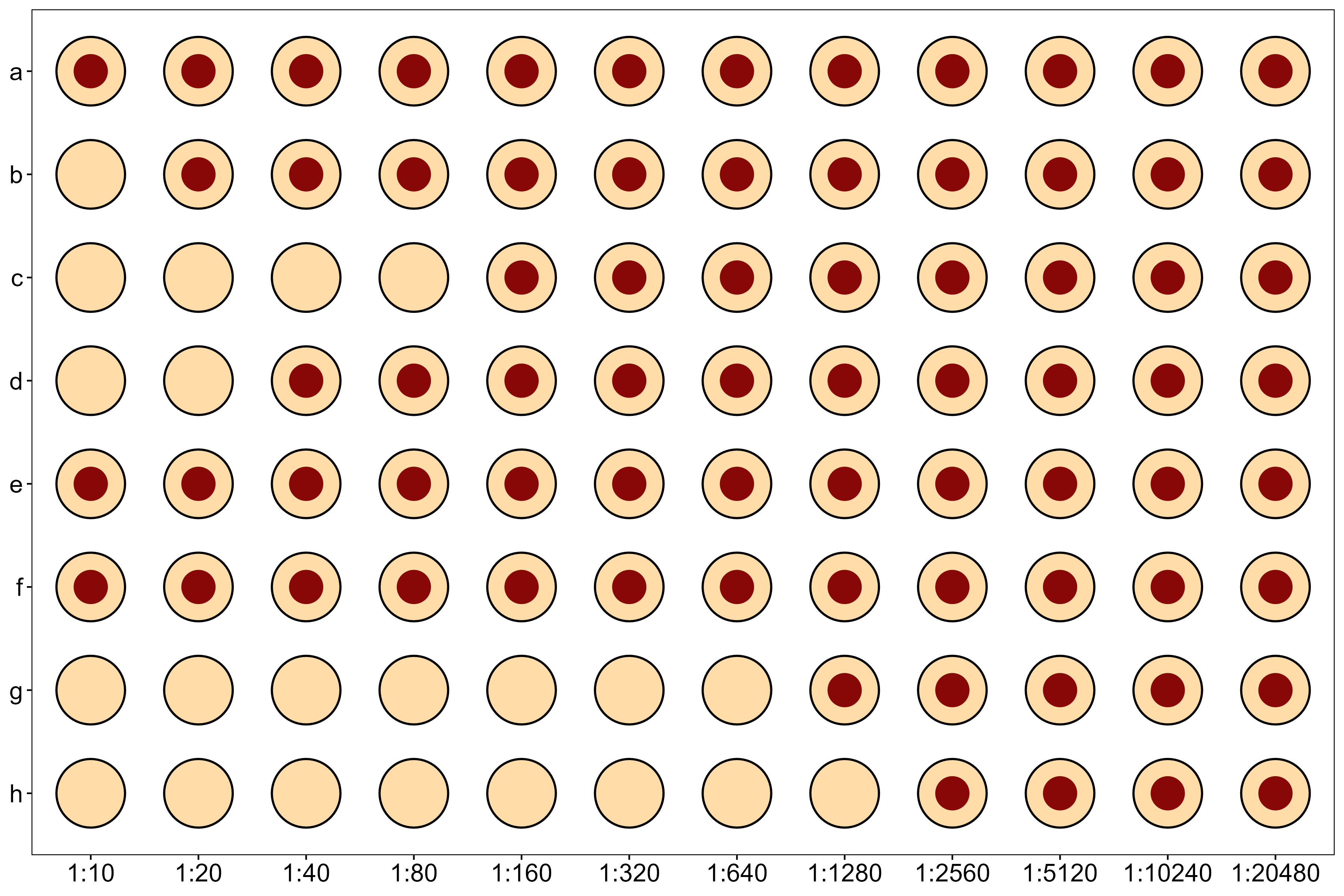
Note also that the measurement process reflects a discretization of an underyling continuous value. The HAI titer measurement is defined as the lowest possible dilution of serum which inhibits agglutination. This value could be, for example, a dilution of 12.5443 (on the natural scale), but we would observe this as a titer of 10 in our assay. Equivalently, the true latent log-scale titer might be 1.327, which we would observe as 1. See Figure Figure 8.1 for an example showing the raw lab assay.

Figure 8.1: Example HAI titer data that we would observe while doing the assay in the lab. These assays are run on 96-well plates, where each row is a separate assay and each column is a serial two-fold dilution, beginning at a dilution of 1:10 (of the serum) and progressing rightwards.

A convenient way to write this is by noticing that we take the floor of all values on the log scale. So, we can write our data observation model as $$\begin{array}{}\text{(8.4)}& y_i=\{\begin{array}{ll}0,& y_i^{\ast }<1\\ \lfloor y_i^{\ast }\rfloor ,& y_i^{\ast }\ge 1\end{array}\end{array}$$

where $y_i^{\ast }$ is the latent true titer and $y_i$ is the observed titer.

8.4 Data simulations

The first thing we need to do now is simulate some titers. We probably want to simulate data from both of those two models, in order to see how the distributions differ. So, we’ll ensure that the linear regression coefficients are the same, and we can see what happens in both models.

8.5 Midpoint correction instead of interval censoring

8.6 Extensions to consider in the future

• An individual is randomly missing strains due to laboratory errors
• Repeated measures across study years
• Repeated measures across study years where some strains are systematically missing based on the year
• Models which control for pre-vaccination titer.